COUNT Function

What is the COUNT Function?

The COUNT function in Excel helps find the number of cells that contain a numerical value. The function will return an integer value for all the cells with a numerical value or arguments containing numbers.

Working in Excel primarily involves lots of number crunching and is used by small businesses to big conglomerates. 

There could be instances where you might not just input the numerical values but also count how many numbers you have input in Excel. 

This article will focus on how you can best use the function by performing numerous counting tasks involving numbers.

COUNT function Formula

This function is categorized as a Statistical function that returns the count for cells with a numerical value. For example, if the range A1:A3 has values 1, 2, and 3, the function will return the result as 3.

However, if the value in cell A1 is replaced by ‘WallStreetOasis,’ the function will return the result for the COUNT function as 2. As cell A1 contains a text value, Excel will ignore the cell and exclude it from the result.

The function will include only the cells in the result that have numerical values such as negative numbers, percentages, date and time, fractions, or even formulas that return numbers. On the other hand, all the empty cells and text strings will be ignored in the result.

The syntax for the function:

=COUNT(value1,[value2]..)

where,

• value1 = (required) reference to cell or range of cells for which we want to count the numbers
• value2 = (optional) additional cell references for which we want to count the numbers

An important thing to remember is that the function will ignore empty cells and text strings in cells and only count those cells with a numerical value.”

How to use the COUNT Function in Excel?

To use the function, you begin with an equal sign (=), type the function name in Excel, and then directly reference the cell or range of cells for which you need to count the numbers.

Example 1

Assume that you have a dataset of numbers from 1 to 10, as illustrated below:

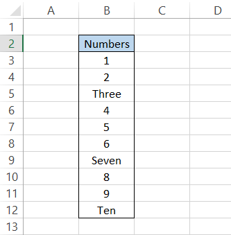
Some numbers are represented in the text, while others are in number format. To count the cells that have a number format, we will use the formula =COUNT(B3:B12), which will give you the result:

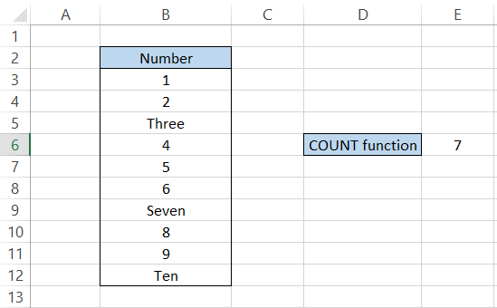
The function returned the result as 7, meaning only those cells had a numerical value while all the other cell values (text) were ignored.

Example 2

We have already emphasized how the function will also include the cells in the result that store values in the form of numbers. This includes date and time, stored as serial and decimal numbers, respectively. 

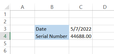
For example, the data is stored as serial numbers in Excel, with 1 representing 1st Jan 1900.

If you need to find the serial number for a specific date, say 7th May 2022, select the cell, press the keyboard shortcut of Ctrl +1, and reformat the cell as a number.  

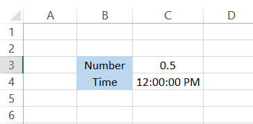
As for the time, a 24-hour clock can also be represented in decimal values between 0 and 1, with 0 representing 12:00:00 AM and 0.9999 representing 11:59:51 PM. 

This means if the decimal value lies between the two ends, i.e., if the value is 0.5, the time is approximately 12:00:00 PM (12 hours time period).  

Since it is clear that both time and date are numerical values, we will see how the function interacts with it and other similar numerical values. 

Assume the data illustrated in the table below. We have eight different types of numerical values represented in the range C3:C10.

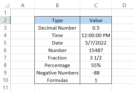
Using the formula =COUNT(C3:C10) in cell C12, we will get the result as 8, meaning 8/8 cells in our table contain a numerical value. 

This includes fractions, percentages, or even the formula =IF(C9<0,1,0) that gives a number as a result, as in cell C10.

COUNT Function Practical Examples

Enough with values that the function would accept and that wouldn't. If one needs to understand Excel functions, related examples are the best way to learn exponentially.

In this section, we will see examples based on real-life scenarios where you might use the function.

Example 1

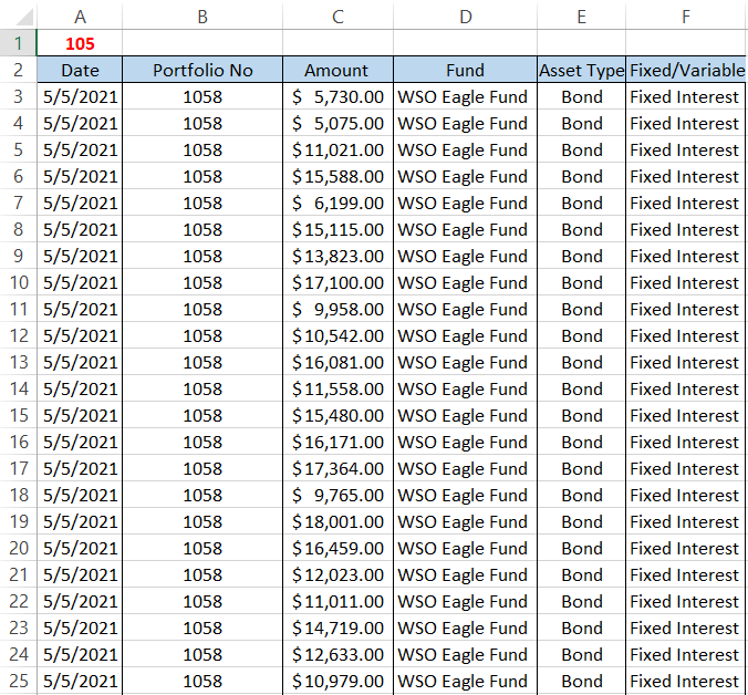
As a financial analyst, you will work on many spreadsheets where the first column consists of dates. 

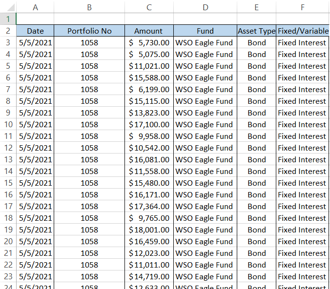
Suppose the email says that the file has 105 rows of data; rather than finding the column with numbers (for example, amounts or price), you can directly use the function on the date column using the formula =COUNT(A3:A108) in cell A1. 

If the count matches that of the email, everything is fine, or you can always revert to clients regarding missing information. 

The dates in the 'Date' column are less likely to go missing (just an assumption!) compared to other columns, particularly 'Amount' or the 'Portfolio No.'

Example 2

Suppose the teacher needs to find the number of exams each student has given in their fall semester. The data looks as illustrated below:

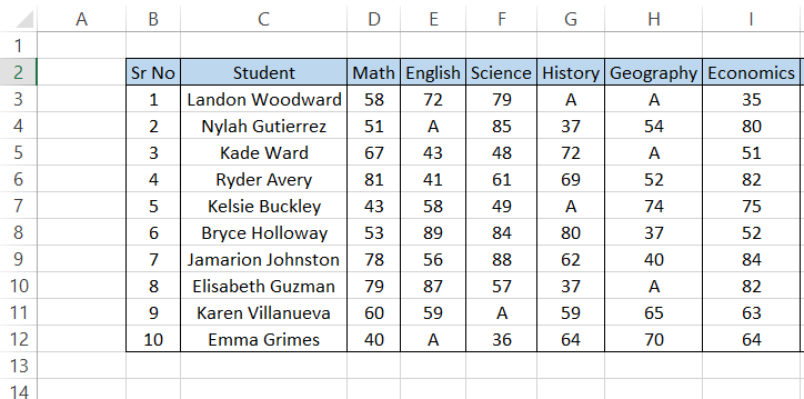
To find the exams submitted by each student, you will use the formula =COUNT(D3:I3) in cell J3 and drag it down to cell J12. The table should look as illustrated below:

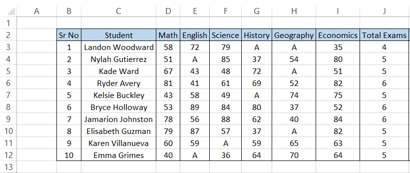
Out of 6 exams, only three students submitted all of them, while the rest missed one examination, along with 'Landon Woodward' who missed his two exams. 

Wherever we can see the alphabet A for 'absent,' the cell ignores that value and returns the result for the rest of the cell.

Remember that the function has nothing to do with adding any numbers present as the cell value. 

Even if you hardcode a value, say the formula becomes =COUNT(D3:I3,589) in cell J3, the result will be 4 + 1 equals five and not 4 + 589 to give 593 as the result of the formula.

COUNT along with IF Function

The one function that works well with COUNT is the IF statements. Of course, we already have the COUNTIF function that returns a result based on user-defined criteria, but that just provides a count. 

However, using COUNT with one or more IF statements gives you more flexibility in terms of the results that you want from Excel.

For example, based on the COUNT result for the student's examination, we can nest the result inside the IF function so that students who haven't submitted all their exams will return as TRUE.

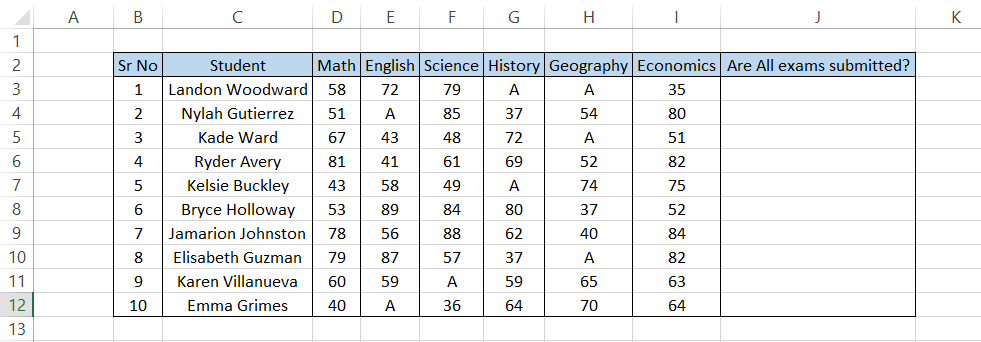
Here, we will use the formula =IF(COUNT(D3:I3)=6, "Yes," "No"), which will give you the result:

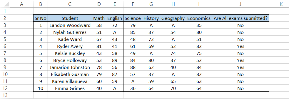
As you can see, wherever we have a test score, the function assigns a value equal to one and then adds them all up to give the final count.

If the student has submitted all of their six exams, we get the result as 'Yes,' while if the student has missed one of their exams, we get the result as 'No.'

Since the COUNT function cannot capture the text string 'A' in our dataset, the IF function evaluates it to FALSE and gives us the corresponding customized result.

Very few functions don't go well with the IF function, and COUNT is not one of them!

General Approach to find the cell 'COUNT'

In general, there might be instances when you need to find the number of cells in a rectangular range. Even though the approach does not use the COUNT function, the result obtained fulfills the purpose of what the COUNT or COUNTA function would do.

Let's say you need to find the total number of cells that have values in the dataset illustrated below:

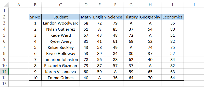
We will use the combination of ROWS and COLUMNS function such that the formula becomes =ROWS(B3:I12)*COLUMNS(B3:I12), which will give you the total cell count excluding the headers as 80.

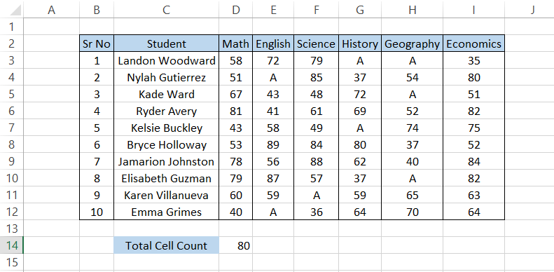
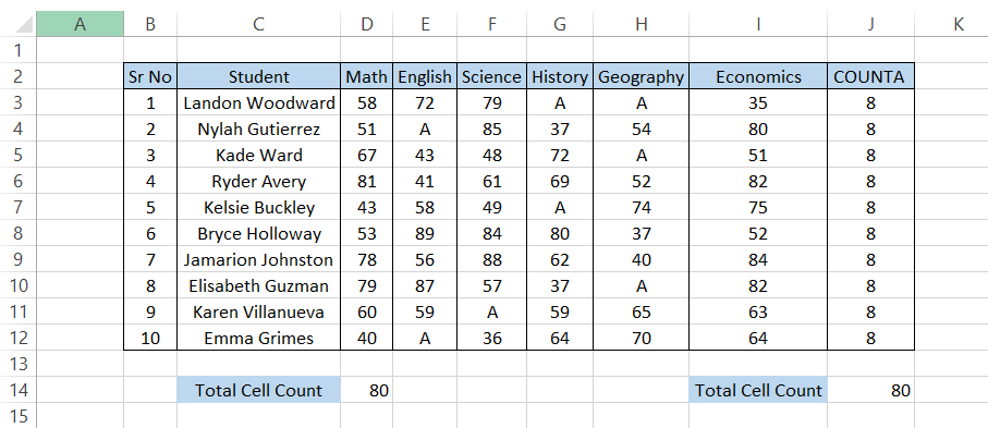
An important thing to remember is that the formula exhibits greater similarity to the COUNTA function that 'counts everything' rather than COUNT. 

Though we have already covered the COUNTA function in an entirely separate article, here, you would have to use the formula =COUNTA(B3:I3) to get the result 8 for each row and then finally add up those numbers to get the result 80, which is quite not an efficient method.

What formula you use to calculate the number of cells entirely depends on you, but remember that if there is more than one way to do a particular task, there is a reason behind it!

Researched and Authored by Akash Bagul | Linkedin

Free Resources:

To continue learning and advancing your career, check out these additional helpful WSO resources:

• SUM Function
• STDEVPA Function
• TIME Function
• VAR.P Function
• YIELD Function