T.INV.2T Function
An Excel Statistical Function that calculates the 2-tailed inverse of the Student’s T-distribution, if the probability of the distribution and the number of degrees of freedom are known.


What Is The T.INV.2T Function?
The T.INV.2T function is an Excel Statistical Function that calculates the 2-tailed inverse of the Student’s T-distribution if the probability of the distribution and the number of degrees of freedom are known.

Where, the Student's t-distribution, or simply t-distribution, is a probability distribution in statistics to make conclusions about the mean of the population in small sample sizes or when the population's standard deviation is unknown.
T.INV.2T function is predominantly used in statistical analysis and hypothesis in small sample sizes.
Some statistical functions in Excel are the NORMINV function and the NORM.S.INV function.
Another interesting statistical function in Excel is the T.INV.2T function. In this article, we will learn about this function from scratch.
- The Student’s T-distribution is a probability distribution that expresses the standard normal distribution in generalized form.
- The Student’s T-distribution helps in machine learning for linear regression and statistical analysis. It also helps to analyze the statistical significance between two population means by the student’s t-test.
- The T.INV.2T function returns the value of the probability distribution function for a Student’s T-distribution in Excel if the probability of the distribution and the number of degrees of freedom are known.
- The T-value for a Student’s T-distribution can either be one-tailed or two-tailed. A one-tailed t-value has only one critical region, while a two-tailed t-value has two critical regions.
Understanding T.INV.2T Function
T.INV.2T is one of the statistical functions in Excel. This function calculates the two-tailed Student's T-distribution. In statistical terms, the Student’s T-distribution is a continuous probability distribution that expresses the standard normal distribution in generalized form.
This distribution is symmetric about zero, and graphically represented in a bell shape, similar to the standard normal distribution. It is used for testing hypotheses on small data sets and in machine learning for linear regression analysis.
The Student’s T-distribution is also used to construct Confidence Intervals between two population means. It also plays a significant role in statistical analysis processes like the Student's t-test for analyzing statistical significance between two sample means.
The probability density function (pdf) of this distribution is continuous, as shown below:

Here:
- t: The continuous random variable,
- v: The number of degrees of freedom, and
- Γ: (greek letter, capital gamma) the gamma function
If v is 1, the Student’s T-distribution becomes the standard Cauchy Distribution. If v tends to infinity, this distribution becomes the standard normal distribution.
NOTE
In financial analysis, the T.INV.2T function in Excel, an upgraded version of the TINV function, helps examine the relationship between a portfolio's risk and return.
The formula of the T.INV.2T function in Excel is as follows:
=T.INV.2T(probability, deg_freedom)
The terms in parentheses are called the function's arguments. The T.INV.2T function uses two arguments which are as follows:
- Probability: This argument refers to the probability corresponding to the Student’s T distribution. The probability of the distribution should lie between 0 and 1. If the probability is less than 0 or greater than 1, the function returns #NUM! Error.
- deg_freedom: This argument refers to the number of degrees of freedom with which the distribution has to be characterized. The number of degrees of freedom should always be more than 1. If the degrees of freedom is less than 1, the T.INV.2T function returns #NUM! Error.
One-Tailed vs. Two-Tailed T-value
There are two ways of calculating statistical significance for a member of a population concerning the test statistic:
- One-Tailed test
- Two-Tailed test

To test hypotheses, we require a test statistic whose distribution is known. There can be two divisions of a probability density curve in a test. They are:
- Region of Acceptance
- Region of Rejection
The region of rejection is known as the critical region. The one-tailed test is a statistical test in which the critical region lies only on one tail. Hence, the one-tailed test has only one critical region. In a one-tailed test, the alternate hypothesis is articulated directionally.
A two-tailed test is a statistical test in which the alternate hypothesis is not articulated directionally. In this test, the critical region is present in both tails. So, a two-tailed test has two critical regions.

Hence, the rejection region appears in both directions of the sampling distribution in a two-tailed test. On the other hand, in a one-tailed test, it appears either on the left or right of the sampling distribution.
In a one-tailed test, the alternate hypothesis has only one end, while in a two-tailed test, it has two ends.
In the following topic, we have discussed examples related to both one-tailed and two-tailed test values to help you understand the two tests and their practical applications.
Example of the T.INV.2T Function
Having reviewed all the theoretical concepts and formulas related to the T.INV.2T function, let's examine some examples to understand and appreciate its practical application in Excel.

Let us take a look at example 1.
Let us assume hypothetical data in which the probability corresponding to the student’s t-distribution is 0.6, and the number of degrees of freedom of the distribution is 4.
The data looks as illustrated below:
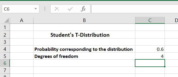
As shown above, in the Excel sheet, cell C4 shows the probability corresponding to the distribution, and cell C5 the number of degrees of freedom.
Using the T.INV.2T function, the following formula is used to get the value of the probability distribution function (pdf) for a probability of 0.6 and 4 degrees of freedom.
=T.INV.2T(C4,C5)
On writing the above formula in cell C7, we get the desired result as shown below:
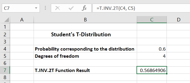
Hence, we get the value of the function as 0.56864906 for the Student’s T-Distribution with a probability of 0.6 and 4 degrees of freedom.
In this way, we can calculate the T-value for any Student’s T-distribution with known probability and degrees of freedom using the T.INV.2T function in Excel.
We determined a two-tailed t-value in the example above. In the next example, we will learn about calculating a one-tailed t-value. This article has already presented a distinction between the t-value with one-tail and the t-value with two-tails in the section above.
Example of the T.INV.2T Function in Excel: Calculating both the one-tailed and two-tailed t-values
We'll calculate both the one-tailed and two-tailed t-values, in this case, to further emphasize the differences.

We have already seen the calculation of the two-tailed t-value in example 1. We use the following formula to compute the two-tailed t-value:
=T.INV.2T(probability, deg_freedom)
We need to replace the probability with 2*probability to calculate the one-tailed t-value. The formula to obtain the one-tailed t-value in Excel is as follows:
=T.INV.2T(2*probability, deg_freedom)
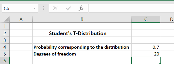
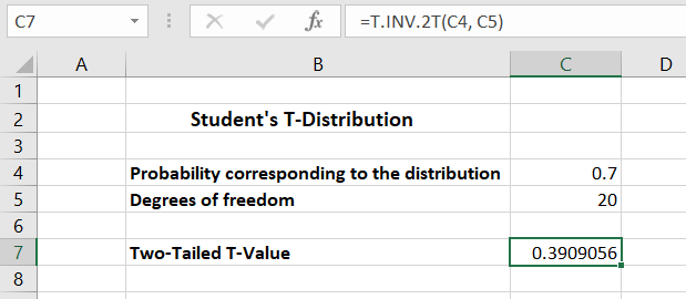
Let's say we have hypothetical data of the Student's T-Distribution with a probability of 0.7 and 20 degrees of freedom. The data looks as shown below:
We can calculate the two-tailed t-value by using the following formula:
=T.INV.2T(C4, C5)
Using this formula, we get the result as shown below:
We use the following formula to calculate the one-tailed t-value for the same probability and degrees of freedom:
=T.INV.2T(2*C4, C5)
On using the above formula in cell C8 of the Excel sheet, we get the one-tailed t-value as shown below:

Hence, in this way, we can calculate the one-tailed and two-tailed t-values in Excel for a Student’s T-Distribution, with known probability and degrees of freedom.

Free Resources
To continue learning and advancing your career, check out these additional helpful WSO resources:


or Want to Sign up with your social account?