Confidence Interval
An estimate of a range that might include a population parameter


What is Confidence Interval?
In statistics, a Confidence Interval estimates a range that might include a population parameter. A sample parameter derived from the sampled data is used to find the unknown population parameter.
Simply put, a confidence interval provides an estimate of the range within which the true population parameter is likely to lie based on sample data and a chosen confidence level.
These intervals generally lie between the upper and lower bounds and are symbolized by percentage. These percentages demonstrate the confidence levels. The confidence level is the long-run fraction of related Confidence Intervals that contain the parameter's real value.
The confidence level, sample size, and sample variability all impact the intervals' s breadth. If everything else remained constant, a bigger sample would result in a narrower confidence range, as larger sample sizes provide more precise estimates of the population parameter.
Similar to how a broader confidence interval is produced by increased sample variability, a wider confidence interval is required by higher levels of confidence.
-
A Confidence Interval in statistics estimates a range that likely includes a population parameter based on sample data and a chosen confidence level.
-
A Confidence Interval estimates where the true population parameter may lie, with the confidence level indicating the likelihood of capturing the true value.
-
Common confidence levels include 90%, 95%, and 99%, with higher confidence requiring larger sample sizes and resulting in wider intervals.
-
Two main types of Confidence Intervals are the Z-interval, used when the population standard deviation is known, and the T-interval, used when the standard deviation is unknown or the sample size is small.
-
Confidence Intervals are calculated using formulas involving the mean, standard deviation, and critical values based on the chosen confidence level and distribution.
-
Misinterpretations include assuming that 95% of the sample data lie within the Confidence Interval or that the Confidence Interval guarantees capturing the true parameter in a specific instance.
Understanding Confidence Interval
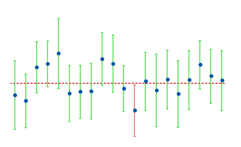
Using the Confidence Interval, a statistician may assess how well research predicts the entire population's behavior. There must be a matching Confidence Interval for every research outcome variable, including success, task duration, number of mistakes, and other parameters.
Although more desired and containing more information, narrow intervals typically call for bigger sample sizes. Because of this, it is doubtful that small research results would accurately reflect all users' behavior.
Where is it used? Researchers use this to assess the level of uncertainty in a sample variable value.
For instance, to determine how each sample could accurately reflect the real value of the population variable, a researcher randomly picks many samples from the same population and computes a confidence interval for each sample.
All generated datasets are unique, with some intervals including the real population parameter and others not.
Confidence Levels
The proportion of potential samples that are anticipated to include the true population parameter, i.e., how frequently you repeat the experiment or resample the population in the same manner, to obtain an estimate that is close to it.
For example, if the confidence level is 99%, then out of a hundred samples taken, 99 of them would have the parameter's true value. The commonly used levels are 90%, 95%, and 99%.
Because it affects your sample size and Confidence Interval, the confidence level you choose is crucial. Your sample size needs to be greater the more confident you wish to be. The larger the Confidence Interval, the more confident you want to be.
Different Confidence Intervals
Two kinds of Confidence Intervals can be used for estimating the mean:
- Z-Interval: When the sample size is greater than or equal to 30, and the population standard deviation is known, or the original population is normally distributed with the population standard deviation known, the z-score is used
- T-Interval: When the Population standard deviation is unknown and the original population is normally distributed, or the sample size is greater than or equal to 30 and the population standard deviation is unknown, the t-interval is used
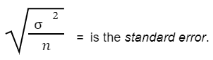
Margin of Error (MOE)
The Margin of Error (MOE) indicates the extent of random sampling error in survey findings is the margin of error. A poll's ability to accurately represent the findings of a survey of the complete population should be questioned the greater the margin of error.
If the outcome measure has a positive variance, the measure fluctuates, or the population is not entirely sampled.
The formula for the Margin of Error is:
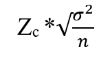
Where,
Zc= is the critical value using the z-score and
But what is the purpose of Confidence Interval? It is termed a measure of uncertainty. This method is often used for research-based projects like clinical trials. It can represent how "acceptable" a trial's estimation is.
There are mainly two ways to derive the interval:
- Traditional approach: This is the historical/mathematical approach of solving the trial data by the use of a statistical T-test
- Computerized approach: This technique is based on bootstrap resampling. Bradley Efron first defined this lucid yet powerful method. A single set of observations is used to generate several resamples (with replacement), and each resamples effect size is calculated

How to Interpret a Confidence Interval
Interpreting the intervals can sometimes be difficult as people phrase it differently. This can be assumed as that there is 99% confidence that the parameter's actual value will fall within the upper limit and the lower limit in the future.
This does not mean:
- That 99% of the trial data lie within the Confidence Interval or
- A determined confidence level of 99% does not always indicate that there is a 99% chance that a trial parameter from a subsequent run of the experiment will fall within this range
How to Calculate Confidence Interval
The steps we can follow are:
- Find the mean of the dataset
- Determine whether the standard deviation is known or unknown
- Obtain the standard deviation using the z-score or the t-test
- Calculate the upper and the lower bounds in accordance with the standard deviation
These illustrations are to be solved using the steps mentioned above. These will include both using a z-score and t-test with different confidence levels.
1. Formula using z-score
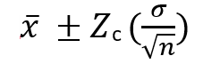
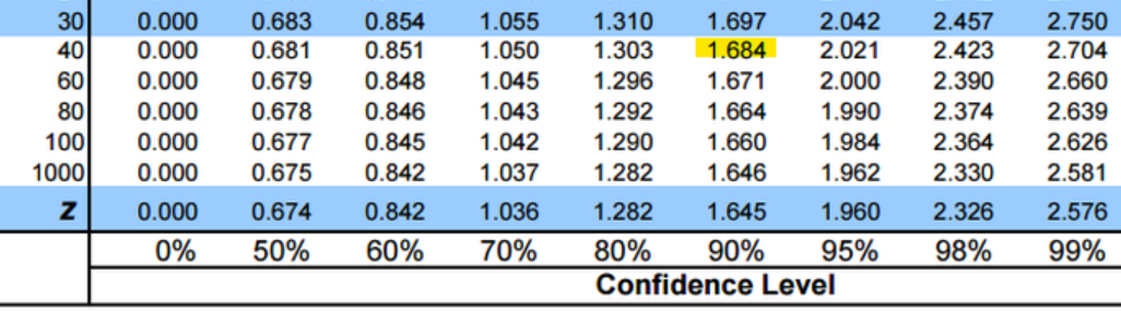
Zc here is the critical value of the confidence level from the normal distribution. The most commonly used critical values are as follows:
| Confidence Level | Critical Values |
|---|---|
| 90% | 1.645 |
| 95% | 1.96 |
| 99% | 2.575 |
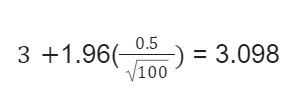
There are 100 cities listed for a survey of college students using radios. The mean of this survey resulted in 3 cities, while the standard deviation was 0.5. Use this information to calculate a 95% confidence interval for the mean of the cities still using radios.
Now, let's calculate:
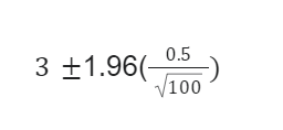
Upper bound:
Lower bound:
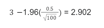
The value of the upper end here would be 3.098, while the value of the lower end is 2.902
In this case, it can be assumed that the survey is 95% certain that the mean of the cities still using radios will fall between 2.902 and 3.098.

2. Formula using T-Interval

Tc here is the critical value from the t-distribution, while s is the standard deviation. In this case, n is the sample size used to determine the degree of freedom (df). The number of values in a statistic's final computation that are subject to change is referred to as its degrees of freedom.
Where,
df = n-1 (n is the sample size)
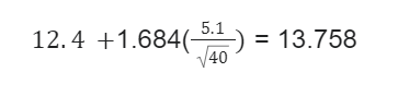
Suppose that a sample of 41 employees at a large company was asked how many hours a week were inefficient. The mean number of hours is 12.4, with a standard deviation of 5.1. Calculate a 90% confidence interval to estimate the mean of the time, which is inefficient per week.
To calculate, we'll use:
n = df = n-1
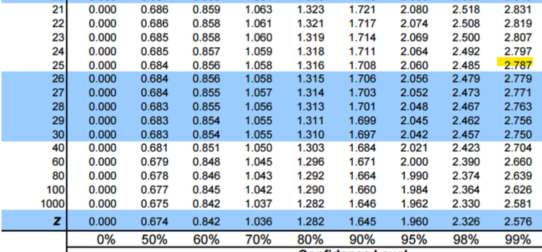
While calculating through t-interval, the critical value is found using the t-table.
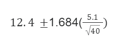
Upper bound:
Lower bound:
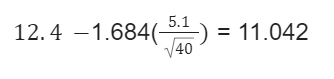
In this case, it will be interpreted that the survey is 90% optimistic that the mean of the inefficient time will fall between 11.042 and 13.758.
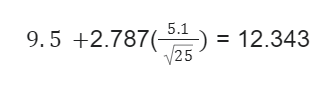
Suppose that there is a drug trial of 26 people for the side effects of the drug. The mean number of hours is 9.5, with a standard deviation of 5.1. Calculate a 99% confidence interval to estimate the mean of the time, which is inefficient per week.
Let's calculate:
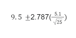
Upper bound:
Lower bound:
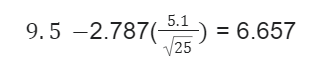
Here, it will be interpreted that the survey is 99% certain that the mean of drug-trialed people for examining the side effects will fall between 6.657 and 12.343.
Confidence Interval Common Mistakes
Generally, it is believed that a 95 percent Confidence Interval does not imply that 99 percent of the data in a random sample falls within these limitations. The range will almost certainly include the population mean, which is what it truly indicates.
Once the interval is constructed, the true parameter is either inside or outside, and no one knows where it falls. We can only state how frequently such intervals may include the genuine mean; this is what confidence level is all about.
This does not imply that 95% of the sample data lie within the confidence interval. Here, there is a 95% certainty that the sample data might fall within the interval's range.
The explanation for this error is rather minor. The important concept relating to a Confidence Interval is that the probability utilized enters the picture with the technique used in calculating it that relates to the method used.
Confidence Interval FAQs
In 1937, Jerzy Neyman introduced Confidence Intervals. At the beginning of the decade, no one realized their importance, but after that, they became a standard for calculating the uncertainties in a dataset.
The value of the test statistic that establishes the upper and lower boundaries of a Confidence Interval or that establishes the level of statistical significance in a statistical test is known as the critical value.
It outlines the distance you must go from the distribution's mean to account for a specific percentage of the overall variation in the data.
These two terms are interconnected but not the same. The Confidence Interval is the range within which the mean of the dataset may lie, whereas the level is the percentage of times you get closer to the assumed value.
There are two methods you may use to determine a confidence interval around the mean of non-normally distributed data:
- To determine it, find a distribution that closely resembles the form of your data
- Find the confidence interval for the changed data after performing a transformation to suit a normal distribution of your data
Although narrow confidence intervals are more desirable and convey more information, they typically call for a higher sample size.
The similarity between Confidence Intervals and hypothesis testing is that both are interpretive procedures that utilize a sample to estimate a population parameter or assess the reliability of a hypothesis.
Confidence intervals are centered on the estimate of the sample parameter for hypothesis tests, whereas hypothesis tests are centered around the null hypothesized parameter.
A t-test is an inferential statistic used to assess whether there is a significant difference between the means of two groups that could be connected to particular characteristics.

Free Resources
To continue learning and advancing your career, check out these additional helpful WSO resources:


or Want to Sign up with your social account?