Correlation
A statistical tool to measure the relationship between two or more variables.


What Is Correlation?
Correlation, in the finance or investment industry, is a statistical tool to measure the relationship between two or more variables, i.e., if the change in one variable results in a corresponding change in the other variables. In other words, this studies whether two variables move in relation to one another.
Cite examples are price and demand, height and weight, and temperature and demand for soft drinks are examples which can be termed to put as correlated.
In finance, it plays an important role because it is used to forecast future trends and manage the risks within a portfolio. In investment, it plays a predominant role in portfolio composition, quantitative trading, and performance evaluation.
The coefficient value ranges between -1.0 and +1.0. In other words, values that range between -1 are termed a negative relationship, and +1 are termed a positive relationship, and the values at or close to zero imply a zero or no relationship.
For example, it could be calculated to determine the correlation between the price of crude oil and the stock price of an oil-producing company, such as Saudi Aramco.
Since oil companies earn greater profits as oil prices rise, the relationship between the two variables is highly positive.
- Correlation measures the statistical relationship between two variables, indicating how one variable moves in relation to the other.
- There are three main types of correlation: positive (both variables move in the same direction), negative (one variable moves up while the other moves down), and zero (no relationship between the variables).
- Correlation is widely used in fields such as finance, economics, psychology, and the natural sciences to identify and analyze relationships between variables, helping to make predictions and informed decisions.
- Correlation does not imply causation; a high correlation between two variables does not mean that one causes the other. Additionally, outliers and non-linear relationships can distort correlation results.
What Correlation Can Tell You
In this article, we shall explain the main three types that tell us about correlation:
-
Positive, Negative, and Zero
-
Linear and Non-linear
-
Simple, Multiple, and Partial
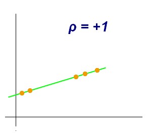
Positive
This happens when r is greater than 0. i.e, +1. It means both variables move in the same direction.
When r is +1, it indicates that the two variables being compared have a positive relationship; if an increase in the value of one variable is interconnected by an increase in the value of other variables, or if a decrease in the value of one variable is interconnected by a decrease in the value of other variables.
| A | 10 | 20 | 30 | 40 | 50 |
|---|---|---|---|---|---|
| B | 80 | 100 | 150 | 170 | 200 |
| X | 40 | 32 | 24 | 16 | 8 |
|---|---|---|---|---|---|
| Y | 25 | 20 | 15 | 10 | 5 |
Example: The relationship between an individual’s height and weight or the relationship between a person’s age and the number of wrinkles.
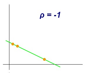
Negative
This happens when r is less than 0, i.e., r is -1. This means both variables move in the opposite direction.
When r is -1, the relationship is said to be negatively correlated: if an increase in the value of one variable is interconnected by a decrease in the value of other variables, or if a decrease in the value of one variable is interconnected by an increase in the value of other variables.
| A | 2 | 4 | 6 | 8 | 10 |
|---|---|---|---|---|---|
| B | 15 | 12 | 9 | 6 | 3 |
| X | 54 | 63 | 72 | 81 | 90 |
|---|---|---|---|---|---|
| Y | 7 | 14 | 21 | 28 | 35 |
Example:
The relationship between an individual’s tiredness during the day and the number of hours they slept the previous night: the amount of sleep decreases as the feelings of tiredness increase.
The more I climb the mountain; it gets colder.
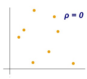
Zero or No
The variables that do not have a relationship with each other. In other words, it demonstrates that it does not have any relationship between both variables.
For example,
The relationship between hours of sleep and shoe size.
The level of the students being bullied and the lower the student’s grades on the standardized tests.
| X | 20 | 5 | 100 | 3 | 80 |
|---|---|---|---|---|---|
| Y | 24 | 65 | 11 | 90 | 2 |
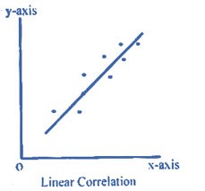
Linear
It’s when the ratio of change between the two sets of variables is the same. For instance, when a 10% increase in one variable is accompanied by a 10% increase in the other variable.
| X | 10 | 15 | 30 | 60 |
|---|---|---|---|---|
| Y | 50 | 75 | 150 | 300 |
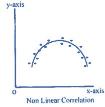
Non-linear
If the amount of change in one variable does not bring the same ratio of change in the other variable, it’s a non-linear correlation. For example, a drug may become more helpful over a certain range but then become harmful.
| X | 2 | 4 | 6 | 8 | 10 |
|---|---|---|---|---|---|
| Y | 8 | 10 | 18 | 22 | 16 |
Simple
This happens only when two variables are studied together. An example is the study of the relationship between price & demand of any product or price and supply.
Multiple
This happens when three or more variables are studied simultaneously. For instance, when we study the relationship between the rice yield per acre with rainfall and fertilizer together.
Partial
Let us assume more than two variables, one dependent variable, and one independent variable, by keeping the other independent variables constant. For example, the yield of rice is influenced by the amount of rainfall and the amount of fertilizer used.
However the studies show the relationship between the yield of rice and the amount of rainfall by keeping the number of fertilizers used constantly.
How to Find the Correlation?
Karl Person is an English mathematician and biostatistician and has been credited with establishing the discipline of mathematical statistics.
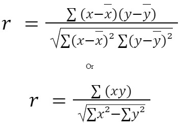
One of the most commonly used methods among algebraic methods of measuring it. It is also known as the Pearson Product Moment Correlation Coefficient (PPMCC), developed in 1896.
This is how we interpret the Coefficient of Correlation:
-
When r = +1, This means there is a positive relationship between variables.
-
When r = -1, This means there is a negative relationship between variables.
-
When r = 0, This means there is no relationship between the variables.
-
When r is closer to +1, This means there is a high degree of a positive relationship between the variables.
-
When r is closer to -1, This means there is a high degree of a negative relationship between the variables.
-
When r is closer to 0, This means there is less relationship between variables.
There are quite a few ways to calculate Pearson's Coefficient of Correlation. This article will cover the three most commonly used methods to account for it.
1. Arithmetic Mean Method
The arithmetic means the method is calculated by taking the actual mean.
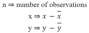
Where
Let us take an example to understand the correlation between age and playing habits among students.
| Age | Number of Students | Regular Players |
|---|---|---|
| 20 | 500 | 400 |
| 21 | 400 | 300 |
| 22 | 300 | 180 |
| 23 | 240 | 96 |
| 24 | 200 | 60 |
| 25 | 160 | 24 |
Let’s take X age and Y percentage of regular players
| Y |
400/500 ×100 =80 |
300/400 ×100 =75 |
180/300 ×100 = 60 |
96/240 ×100 = 40 |
60/200 ×100 = 30 |
24/160 ×100 = 15 |
|---|
Let’s put the sum into the calculation
|
Age (x) |
Regular players (y) |
x - x ̅ (X - 22.5) |
y - y ̅ (Y - 50) |
(x - x ̅) * (y - y ̅) | (x - x ̅)² | (y - y ̅)² |
|---|---|---|---|---|---|---|
| 20 | 80 | -2.5 | 30 | -75 | 6.25 | 900 |
| 21 | 75 | -1.5 | 25 | -37.5 | 2.25 | 625 |
| 22 | 60 | -0.5 | 10 | -5 | 0.25 | 100 |
| 23 | 40 | 0.5 | -10 | -5 | 0.25 | 100 |
| 24 | 30 | 1.5 | -20 | -30 | 2.25 | 400 |
| 25 | 15 | 2.5 | -35 | -87.5 | 6.25 | 1225 |
| 135 | 300 | -240 | 17.5 | 3350 |
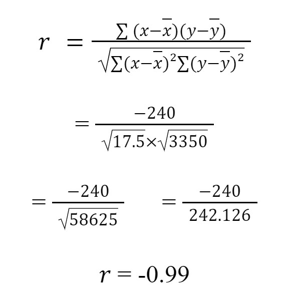
In this example of the age and playing habits among students from the 20-25 yrs old category, we divided the regular player by the total number of students among each age category (80,75,60,40,30,15) and applied it to corresponding ages.
Age has been denoted as x and y as regular players.
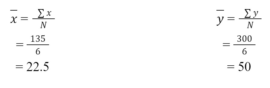
Then take the mean (sum total of x divide it with total observations (6) >> (x =22.5), same as with y >> (y = 50)), and subtract it on x & y each. Since we got the values of x-x & y-y, We then multiplied it (-240) and took squares of x (17.5) and y (3350).
Finally, applied the formula x-x * y-y, dividing the whole by finding the square root of 58625 as 242.126 and then dividing -240 with 242.126 and got a result with a negative relationship of -0.99.
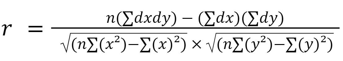
2. Assumed Mean Method
The assumed mean method is calculated by taking the assumed mean only.
Let us take an example to understand the correlation between size and defectiveness in the quality of the material.
| Size | Number of materials produced | Number of defectives |
|---|---|---|
| 15 | 200 | 150 |
| 16 | 270 | 162 |
| 17 | 340 | 170 |
| 18 | 260 | 180 |
| 19 | 400 | 180 |
| 20 | 300 | 114 |
Let's take,
x ⇒ size (i.e., mid-values)
y ⇒ percentage of defectives
| X | 15.5 | 16.5 | 17.5 | 18.5 | 19.5 | 20.5 |
|---|---|---|---|---|---|---|
| Y |
150/200 ×100 = 75 |
162/270 ×100 = 60 |
170/340 ×100 = 50 |
180/260 ×100 = 50 |
180/400 ×100 = 45 |
114/300 ×100 = 38 |
| x | y | dx | dy | dxdy | dx2 | dy2 |
|---|---|---|---|---|---|---|
| 15.5 | 75 | -2 | 25 | -50 | 4 | 625 |
| 16.5 | 60 | -1 | 10 | -10 | 1 | 100 |
| 17.5 | 50 | 0 | 0 | 0 | 0 | 0 |
| 18.5 | 50 | 1 | 0 | 0 | 1 | 0 |
| 19.5 | 45 | 2 | -5 | -10 | 4 | 25 |
| 20.5 | 38 | 3 | -12 | -36 | 9 | 144 |
| 3 | 18 | -106 | 19 | 894 |
Let's take the assumed mean,
- x = 17.5
- y = 50
- n = 6
Let's apply the formula,
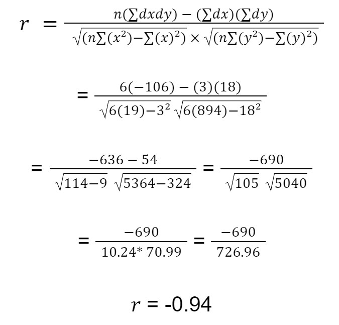
In this example, between size and defective in the quality of the material, we examined the size from 15-20 and divided the number of defects by the total number of materials produced (75,60,50,50,45,38), and applied it to the corresponding size.
Size has been denoted as x and y as the number of defectives.
Then take the mean (sum total of x divide it with total observations (6) >> (dx = 3), same as with y >> (dy = 18)) and subtracted it on x & y each. Since we got the values of dx & dy (-106) we then multiplied it and took squares of dx (19) and dy (894).
Finally, applied the formula and multiplied the number of observations with dxdy and subtracted dx & dy, and divided the whole by finding the square root of 105 & 5040 as 10.24 & 70.99 and got a result of 726.96 and then divided -690 with 726.96 and got a result with a negative relationship -0.94.
3. Direct Method
The calculation happens without taking the actual mean or assumed mean when using this method.
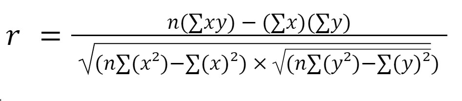
Where n ⇒ number of observations
Let us take an example to understand the correlation between price and demand for different chocolates.
| Price | Demand |
|---|---|
| 10 | 40 |
| 12 | 41 |
| 14 | 48 |
| 15 | 60 |
| 19 | 50 |
Let’s solve
- x = price
- y = demand
| Price | Demand | xy | x2 | y2 |
|---|---|---|---|---|
| 10 | 40 | 400 | 100 | 1600 |
| 12 | 41 | 492 | 144 | 1681 |
| 14 | 48 | 672 | 196 | 2304 |
| 15 | 60 | 900 | 225 | 3600 |
| 19 | 50 | 950 | 361 | 2500 |
| 70 | 239 | 3414 | 1026 | 11685 |
n ⇒ 5
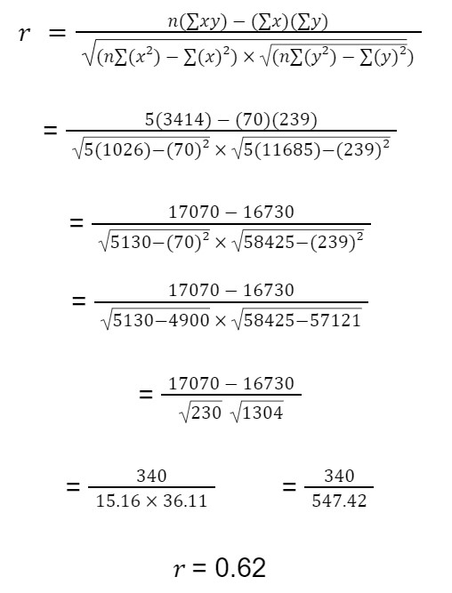
In this example of the price and demand for different chocolates, we examine the price and the demand for each chocolate. Price has been denoted as x (70) and demand as y (239).
We then multiplied the price and demand (3414) and took x² (1026) and y² (11685).
Finally, applied the formula and multiplied the number of observations by XY and, subtracted x & y, and divided the whole finding the square root of 230 & 1340 and got a result as 15.16 & 36.11 and got a result of 547.42 and then divided 340 with 547.42 and got a result with a positive relationship 0.62.

Spearman's Rank Correlation
This method is applied when the variables are measured in a quantitative form. However, there were several cases where measurement was not possible because of the qualitative nature of the variable.
For instance, it's impossible to compare beauty, character, intelligence, honesty, wisdom, etc., quantitatively.
Nonetheless, it is possible to rank these qualitative features in some order. It is obtained from the ranks of the variables instead of their quantitative measurement.
This method was invented by Charles Edward Spearman in 1904, and the name was derived after his name, Spearman's rank correlation coefficient.
This is how we can interpret Spearman's Coefficient:
-
When r = +1, This means it is a perfect positive association between ranks.
-
When r = -1, This means there is a perfect negative association between ranks.
-
When r = 0, This means there is no association of ranks.
-
When r is closer to 0, This means weaker is the association between the two ranks.
The formula is as follows:
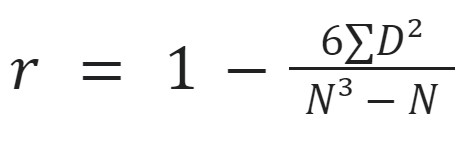
Where
- D = Difference of rank in two series ( denoting as x & y)
- N = Number of observations
Let’s assume the rank correlation coefficient between ten students whose results in a class test of finance and economics are determined.
| Finance | Economics | R1 | R2 | D = R1 – R2 | D2 |
|---|---|---|---|---|---|
| 17 | 36 | 1 | 2 | 1 | 1 |
| 13 | 46 | 5 | 1 | 4 | 16 |
| 15 | 35 | 3 | 3 | 0 | 0 |
| 16 | 24 | 2 | 5 | 3 | 9 |
| 6 | 12 | 10 | 8 | 2 | 4 |
| 11 | 18 | 7 | 7 | 0 | 0 |
| 14 | 27 | 4 | 4 | 0 | 0 |
| 9 | 22 | 8 | 6 | 2 | 4 |
| 7 | 2 | 9 | 10 | 1 | 1 |
| 12 | 8 | 6 | 9 | 3 | 9 |
| 44 |
N ⇒ 10
D ⇒ R1-R2
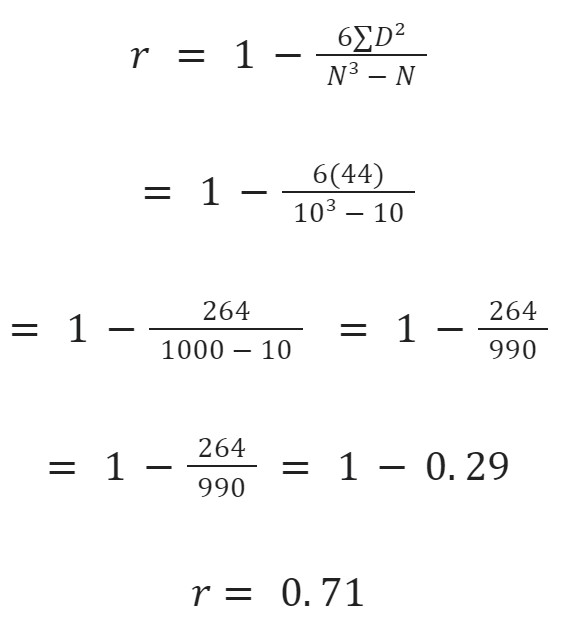
In this example, between 10 students whose results in a class test finance and economics, we tested the intelligence of 10 students. We then examine their ranks in ascending order and arrange them R1 as finance and R2 as economics.
We then subtracted R1 - R2 to get D and take its square D² equals 44.
Finally, we applied the formula and multiplied 6 with D² (264) and divided the number of observations cube (1000) by the number of observations (10), resulting (990) and got a result of (0.29) and subtracted 1 with it which results to a positive relationship 0.71.
Equal Ranks
When ranks are equal, there are chances of obtaining the same ranks for two or more items at a time. When this happens, we take the mean or average of the ranks that are the same. It is even called tied ranks.
To calculate, we rank the tied numbers as if they were not tied, then add up all the ranks they would have and divide it by how many there are.
For instance, in a spelling test, if two observations for the 4th rank, each of those observations should be given in the rank 4.5 (i.e., 4+52=4.5 ). Suppose four observations got 6th rank. Here we have to assign the rank 7.5 (i.e., 6+7+8+94=7.5) to each of the four observations.
The formula For Equal Ranks is as follows:
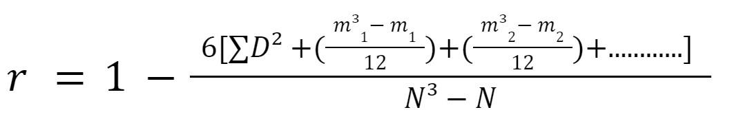
Where
- D - Difference of rank in two series
- N - Total number of observations
- m - Number of times each rank is repeated
Let's take an example to understand this better.
| Marks in Commerce | Marks in Math |
|---|---|
| 15 | 40 |
| 20 | 30 |
| 28 | 50 |
| 12 | 30 |
| 40 | 20 |
| 60 | 10 |
| 20 | 30 |
| 80 | 60 |
In this example of marks in commerce and math, we can see rank repetitions.
For commerce, 20 is repeated twice, corresponding to ranks 3 and 4. Therefore, three is assigned for ranks 2 and 3 with m1 = 2.
For Math, 30 is repeated thrice, corresponding to rank 3,4,5. Therefore, four is assigned for ranks 3,4,5 with m2=3
| Marks in Commerce | Marks in Math | R1 | R2 | D = R1 – R2 | D2 |
|---|---|---|---|---|---|
| 15 | 40 | 2 | 6 | 4 | 16 |
| 20 | 30 | 3.5 | 4 | 0.5 | 0.25 |
| 28 | 50 | 5 | 7 | 2 | 4 |
| 12 | 30 | 1 | 4 | 3 | 9 |
| 40 | 20 | 6 | 2 | 4 | 16 |
| 60 | 10 | 7 | 1 | 6 | 36 |
| 20 | 30 | 3.5 | 4 | 0.5 | 0.25 |
| 80 | 60 | 8 | 8 | 0 | 0 |
| 81.5 |
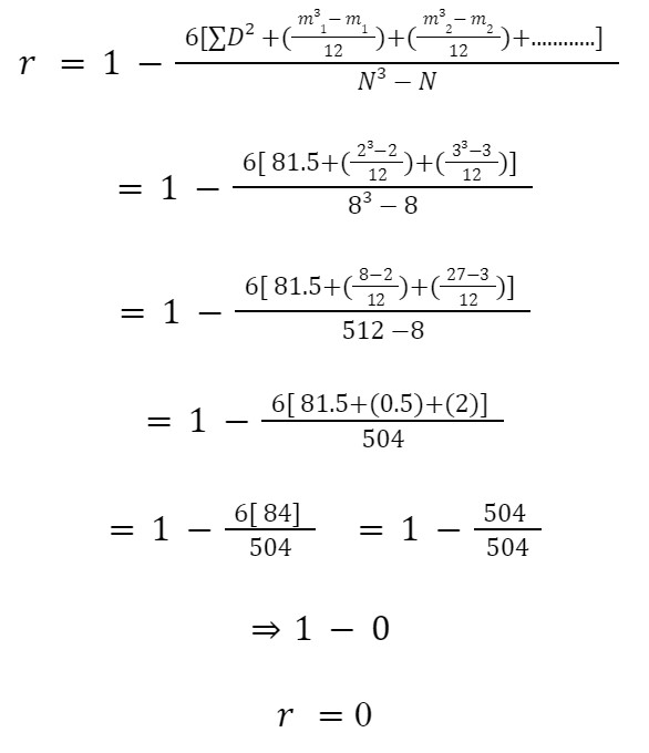
Hence, marks in Commerce and Mathematics are uncorrelated.
From this example of marks in commerce and math, we tested the knowledge of 8 students. We then examine their ranks in ascending order and arrange them R1 as commerce and R2 as math.
We then calculated repeated ranks as mentioned above and subtracted R1 - R2 to get D and take its square D² equals 81.5.
Finally, we applied the formula and multiplied 6 with D² (504) and divided the number of observations cube (512) with a number of observations (8), resulting in (504) and got a result of (0) and subtracted 1 with it which results to an uncorrelated 0.


Free Resources
To continue learning and advancing your career, check out these additional helpful WSO resources:


or Want to Sign up with your social account?