AREAS Function
An Excel function that allows the user to return the count of all the referenced areas in the spreadsheet.


What Is The AREAS Function In Excel?
The AREAS function in Excel allows the user to return the count of all the referenced areas in the spreadsheet. It is common for Excel enthusiasts to be unsure about its actual use case and functionality.
Let’s take an example to understand how the function can improve data analysis in Excel. Suppose you have the range A3:E14, which requires evaluation for a specific ‘lookup’ value.
Even in the lookup range A3:E14, we only have values in columns A, B, and E, while C and D do not have any values. As you know, if there are inconsistencies in the dataset, anyone can make the silliest mistakes.
In this case, you can make a named range of A3:A14, B3:B14, and E3:E14 and then use it with the INDEX function to return a particular value from the named range.
That’s quite a lot of information already, even before we understand what exactly is the AREAS function. Still, let's head to the next section and understand the function and how to use it, along with a couple of examples.
- The AREAS function is a Lookup/Reference function used to count the number of areas in a reference with multiple non-contiguous ranges.
- Users provide a reference containing multiple non-contiguous ranges as the argument to the AREAS function. It returns the number of separate areas within the reference.
- Potential errors that users might encounter when using the AREAS function, such as providing invalid references or referencing cells with incorrect data, and how to address them effectively.
- The function is commonly used in data analysis tasks, such as identifying and categorizing different data sections within a larger dataset by counting the number of separate areas in a reference.
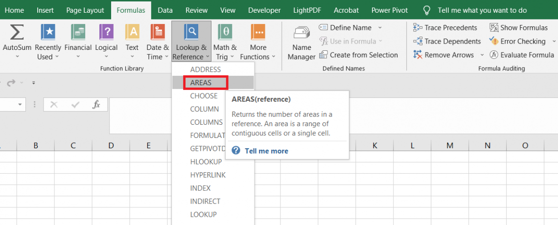
Understanding The AREAS Function
The AREAS is categorized as a Lookup and Reference function that returns the count of areas in the reference.
An area refers to either a single cell or a range of contiguous cells referenced in the function.
For example, the range A1:A3, A4:B4, and A6:B8 are all from different areas in the spreadsheet. The function will eventually identify them as a separate entity and return their number to the user using the AREAS function.
The syntax for the AREAS function is:
= AREAS(reference)
where,
- reference: (required) cells or the range of cells that will be referenced in the function
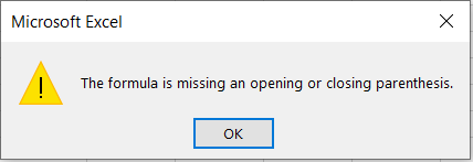
The function allows you to reference multiple ranges of cells easily. However, you need to ensure that you enclose the multiple ranges in an additional parenthesis, or else the function returns an error.
Looking at an example will probably make things a lot easier. Using the function isn't rocket science, but as we said earlier, additional parentheses will make the function work if you make more than one cell reference.
Example of the Areas Function
The function returns the ‘n’ number of referenced ranges in the spreadsheet. For example, if you reference three different ranges of cells, then the result of the function will be 3.
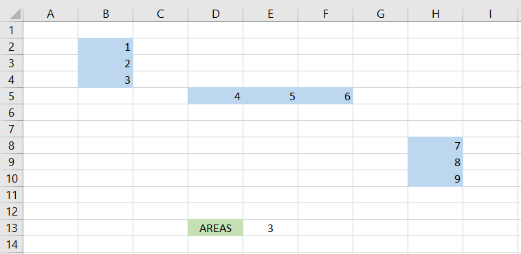
Suppose we have the data as illustrated below:
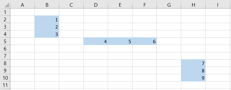
First, let's try to reference just a single range B2:B4 in the function. We will use the formula =AREAS(B2:B4) in cell E13, which gives the result:
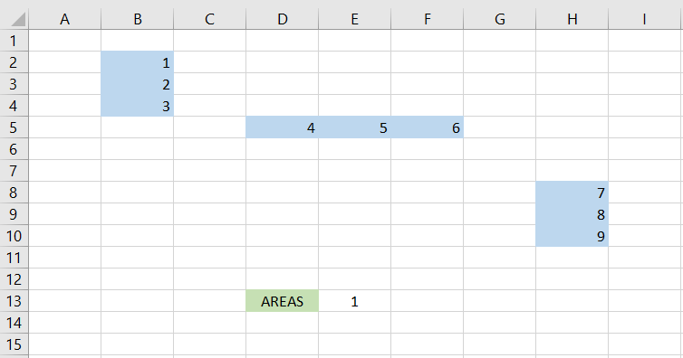
That makes sense, right? We just referenced a single range; hence, the function returns 1 as the result.
Next, let’s try and reference multiple highlighted ranges in the function. The formula will be =AREAS((B2:B4,D5:F5,H8:H10)), giving the result as 3.
If we hadn’t used the additional parentheses in the formula, then Excel would have returned a pretty obvious error:
Once this error is resolved, you will get the expected result in cell E13: 3. And that is how the AREAS function works, ladies and gentlemen.

Uses of AREAS function in Excel
How could the AREAS function be used differently? Well, there are a couple of other ways that you can use the AREAS function. This section of the article will guide you on how you can harness the full potential of the function.

a. Dynamic Named Ranges
The AREAS function can be used along with other functions, such as INDEX and OFFSET, to create a dynamic named range. These ranges automatically adjust in size depending on the number of areas referenced in the formula.
Dynamic named ranges can be useful when you are working on changing data ranges and still want to ensure you cover all the required cells.
Suppose we have two ranges, B2:C4 and E2:F4, as highlighted in the spreadsheet below:
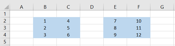
To create dynamic named range, we will use the formula =INDEX($B$1:$E$3,1,1):INDEX($A$1:$E$3,ROWS($A$1:$E$3),COLUMNS($A$1:$E$3)) and press the Ctrl + Shift + Enter key, which gives the result as 1.
The formula will dynamically adjust to cover the entire range containing both areas, i.e., B2:C4 and E2:F4, respectively.
Ensure that the range reference $B$2:$F$4 change according to the actual data.
b. Conditional Formatting
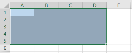
Suppose you have a range of cells from A1:D5 and want to evaluate whether the cells belong to a single area or multiple areas.
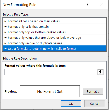
To use the conditional formatting tool, we will click on Home > Conditional Formatting > New Rule, which opens the below window:
Next, we will navigate all the to the ‘Use a formula to determine which cells to format’ and input the formula =AREAS(A1:D5) = 1. We will also use the cell fill option to highlight those cells that fit the mentioned criteria.
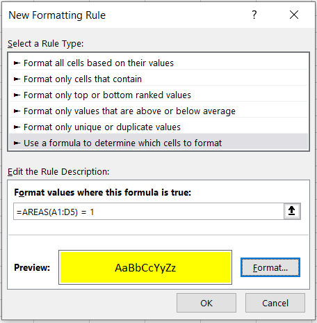
The above formula will check for all the cells where the number of areas equals 1. If the formula evaluates to TRUE, it will highlight those particular cells.
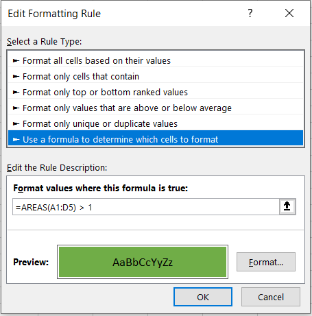
Additionally, we will also create another rule for range A1:D5, where the formula will be =AREAS(A1:D5) > 1, which will check if the number of areas is greater than 1. It means that such cells belong to multiple areas.
After clicking on OK, we will get the result:
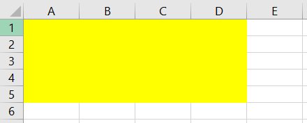
Thus, we can interpret that all the cells in the selected range belong to a single area which is why we have the yellow color cell fill.
c. Array Formula
The AREAS function can also be used to perform different calculations based on the number of references in the formula.
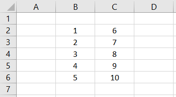
For example, suppose we have the data as illustrated below:
We will use the formula =IF(AREAS((B2:B6, C2:C6)) = 1, SUM(B2:B6), AVERAGE(C2:C6)) in cell E4, which gives the result as 8.
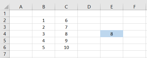
Here, if the range consists of a single area, i.e., both ranges are adjacent to each other, then the formula will calculate the sum of B2:B5. In contrast, if the range consists of multiple areas, then the function calculates the average of C2:C5.
Since we get the result as 8, on closer inspection, we find that this is the average of all the numbers from 6 to 10.
An important thing to remember while using the function is that since this is an array formula, you need to press the Ctrl + Shift + Enter key to return the result in cell E4.

Free Resources
To continue learning and advancing your career, check out these additional helpful WSO resources:


or Want to Sign up with your social account?