DATE Function
An Excel Date/Time function that returns the date based on the numbers you input for the day, month, and year components.


What Is The DATE Function?
The DATE function is an Excel Date/Time function that returns the date based on the numbers you input for the day, month, and year components.
A date in question would always only have three components -
- what day does the event fall on,
- in which month would the event take place, and
- in what year will/was the event be executed?
Based on the intersection of these three parameters, an event is understood to take place on a particular day.
For example, the 4th of July is celebrated as the birth of American Independence each year. However, the original event occurred on 4th July 1776, when the 13 North American colonies declared separation from Great Britain.
Thus, dates, in general, hold great significance in remembering events, irrespective of whether they are small or large. Excel’s ability to accept date values and even have a highly compatible function exhibits the importance of such events.
In this article, we will learn about the DATE function and how to use it, along with a couple of examples.
- The DATE function in Excel is a date-and-time function that creates a date by specifying the year, month, and day. It returns a serial number representing the date in Excel's date system.
- The syntax for the DATE function typically includes three arguments: year, month, and day. It returns a date value based on these arguments.
- The DATE function may return errors if any of the arguments are invalid or out of range. For example, if the month argument is less than 1 or greater than 12, or if the day argument is invalid for the specified month, the function may return a #VALUE! error.
- Excel stores dates as serial numbers, with January 1, 1900, represented by serial number 1. Dates are stored sequentially, with each subsequent day represented by the following sequential number.
How The DATE Function Works
DATE is categorized as a date-and-time function that returns the date based on the numbers input for the day, month, and year components.
First, there are no restrictions on what numbers can be input for date and month components.
However, it's best if we stick with some rules, or the results returned by the function can become quite confusing.
A month can have a maximum of 31 days, whereas a year would only have 12 months. Thus, if possible, ensure that you do not input days greater than 31 or months greater than 12.
What about the year?
Although you can input any date in Excel, the value 1st Jan 1900 is actually the first stored as a serial number in Excel. For example, 1st Jan 1900 is stored as 1, 2nd Jan 1900 is stored as second, and so on.
Thus, you can input all the numbers that fulfill the criteria of 0 ≥x≥ 9999.
Thus, if you have three numbers as 2021, 11, and 21, the result using the function would be 21st November 2021.

Excel is extremely good at identifying whether the format you are using for the date is correct or wrong. If a wrong formatted date is used with other date and time functions, it can give you misleading results or even an error.
What if we input a month greater than 12 or even a day more significant than 31? For now, let's focus on the basics and return to the question when we cover this example.
This is where the DATE function comes in.
The syntax for the function is
=DATE(year, month, day)
where,
- year - (required) number for the year between 0 ≥x≥ 9999.
- month - (required) number for the month
- day - (required) number for day
Note
The function accepts each component only in the order mentioned in the syntax. Also, there is no limit on what numbers you can use for each element.
The function will only return an error when the date returned is smaller than 1st January 1900 and greater than 31st December 9999.
How to Use The DATE Function?
You can use the DATE function in two ways -
- from the function’s library or
- as a worksheet formula.
You can use either method by hardcoding the values or referencing the cells with the numerical values corresponding to each date component.
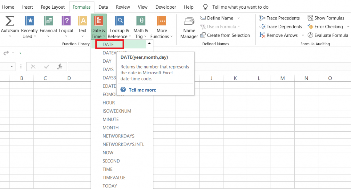
Suppose you want to input the date 21st January 2022. Select the cell where you intend to get the result > click on Formulas > Date and Time > DATE function. We input the numbers for the date as follows:
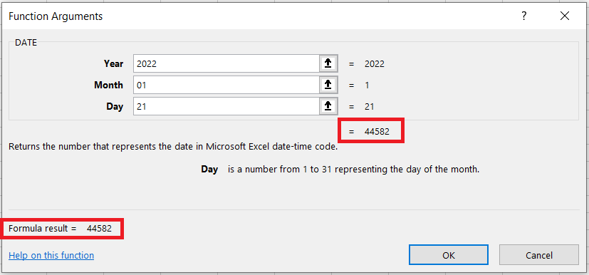
Initially, we get the serial number for the corresponding date, but when you click OK, you will find that the cell value equals 21st January 2022. The format can be different such as 01/21/2022, which you can format anytime to get the desired result.
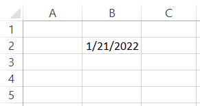
Another way you can get the same result is by using the worksheet formula. In cell B2, we will use the formula =DATE(2022,1,21), which gives a similar result as:
Hardcoding the numbers or simply referencing the cell, the function works similarly.
Example of the DATE Function
In this section, we will see a couple of examples of how to use the function in Excel. Remember, it's okay to input dates using the part. However, it ensures that the dates you have used are in a suitable format.
This way, wherever you reference those date values, whether it be another formula or just finding the difference between two dates, stay assured that what you are doing is correct.
a. Referencing the cells to return date.
Suppose that you have the date components in Excel as illustrated below:
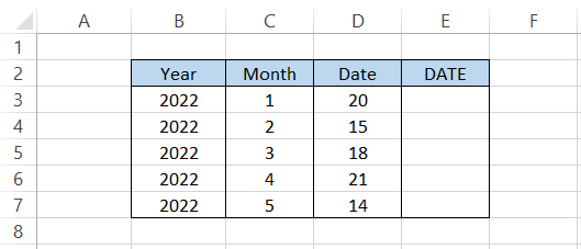
To get the dates, we will use the formula =DATE(B3,C3,D3) in cell E3 and drag it down till cell E7, which gives the result:
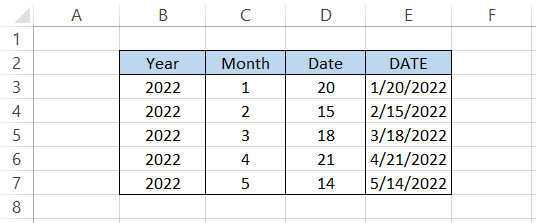
By using the formula, you don’t need to worry if the date you have input is a correct mm-dd-yyyy format.
Even if your local computer accepts dates in dd-mm-yyyy format (yes, all these date formats can be pretty confusing since they are different in different organizations), the DATE function ensures that you do not input wrong data in spreadsheets.
b. Counting the number of dates greater or less than the given date
The COUNTIF function in Excel counts the number of referenced cells based on predefined criteria. For example, If there are ten cells and each cell is to be evaluated if it is empty, then COUNTIF can be used to find the number of empty cells.
All the cells that evaluate the TRUE condition will be counted cumulatively to get the final number in the spreadsheet. The same logic can also be applied to dates. Suppose that you have the data as illustrated below:
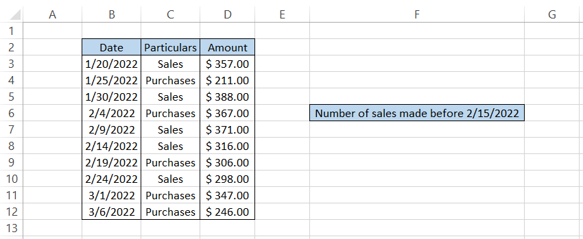
We need to determine how many sales were made before 15th February 2022. A COUNTIF can only accept one condition; however, here we have two - deals and a date, i.e., 15th February 2022.
Thus we will use the COUNTIFS function using the formula =COUNTIFS(B3:B12,"<"&DATE(2022,2,15),C3:C12, "Sales"), which gives the count of sales made before 15th February as 4.
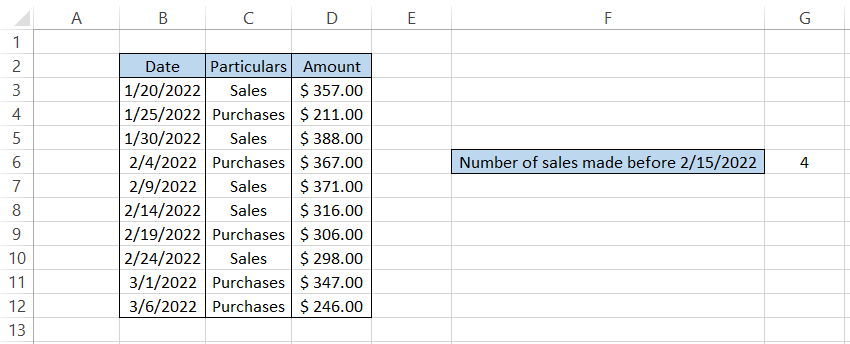
The conditions act as a double filter to exclude the data that does not match and only count the cells where both the conditions evaluate TRUE.
c. Effect of more significant numbers on the date.
The year component will likely show the least volatility since it will be between 0 and 9999. If you input a number smaller or more significant than those respectively, the function will return an error.
What about the days and months? We did ask a question regarding this.
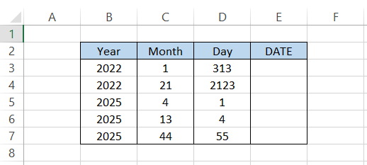
We see that the month and day values are far beyond the 12 and 31-day rule that we had suggested.
If we use the formula =DATE(B3,C3,D3) in cell E3 and drag it down to cell E7, we get the result:
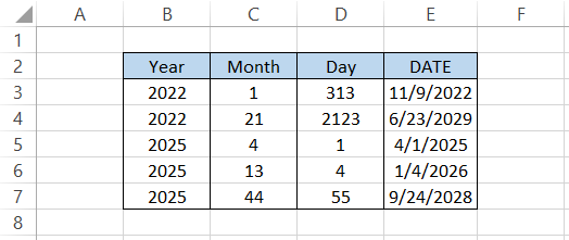
You see, even though we input the month as 1, the value of the month we get in the final result equals 11. This is because the days spread out evenly over several months, which is why the final date is much different than the expected result.
A similar scenario can be seen for the rest of the date values, wherever the month and date values exceed the 12 and 31 numbers, respectively.

DATE Function With Other Date & Time Functions
The functions that work well with the DATE are the other functions present in the Date and Time library.
The various functions that you would find in the library are
- DAY
- DAYS
- MONTH
- YEAR
- EDATE
- EOMONTH
- WEEKDAY
- YEARFRAC, etc.
All these functions have one similar argument, i.e., the date.
In this section, we will see a couple of examples of how you can combine those functions with DATE to ensure the best integrity of date values.
a. DAY, MONTH, and YEAR function
If you need to extract a day, month, or year from a given date, then you can use either of those functions directly.
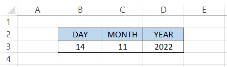
For example, suppose that you have the date as 14th November 2022. To extract the day, we will use the formula =DAY(DATE(2022,11,14)) which gives the result:
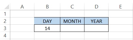
Similarly, you can use the =MONTH(DATE(2022,11,14)) and =YEAR(DATE(2022,11,14)) which gives the result:
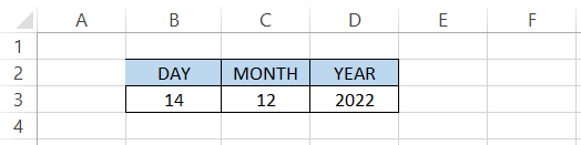
Since we are using the DATE function, you can input any numbers, and the function will still return the month and day by spreading out the days evenly.
For example, if we use the formula =MONTH(DATE(2022,11241,1564)) in cell C3, we get the result as:
b. YEARFRAC
The YEARFRAC function returns the result between two dates in terms of a decimal number.
This function can mainly be helpful in financial modeling when trying to find out the cash flows applicable from the date of investment in a stock or a bond.
The function accepts two required arguments, i.e., the start_date and the end_date, to return the fractional number.
Suppose that you need to find out how much percentage of the year is still remaining based on a given date. The data looks as illustrated below:
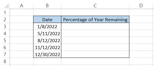
We will use the formula =1-YEARFRAC(DATE(YEAR(B3),1,1),B3) which gives the result:
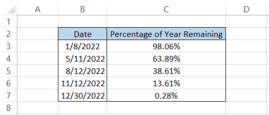
When the date is 8th January 2022, there is still 98.06% of the year remaining, whereas when the date is equal to 30th December 2022, the percentage of the year remaining is equal to 0.28%.
c. DATEDIF
DATEDIF is another function where the DATE function can input the dates in the correct format. The function returns the number of days between two different dates.
Suppose you are looking to find the number of days between 1st January 2022 and a series of other dates. The data looks as illustrated below:
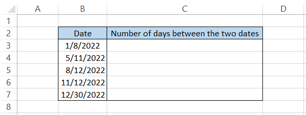
We will use the formula =DATEDIF(DATE(YEAR(B3),1,1),B3, "D"), which gives us the number of days between the two dates as:
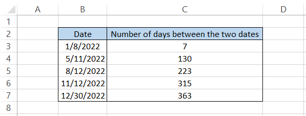
If we want the difference between the two dates in terms of months, we can tweak the formula slightly so that it becomes =DATEDIF(DATE(YEAR(B3),1,1), B3, "M") to give the result:

What we did is only change the unit argument from ‘D’ to ‘M,’ which equals to month. You can even change it to year by changing the value to ‘Y.’
d. NETWORKDAYS
The final function that works really well with DATE is the NETWORKDAY.
The NETWORKDAY returns the number of whole workdays between two given dates. Suppose I need to calculate the workdays between 1st January 2022 and a bunch of other dates.
The data looks as illustrated below:
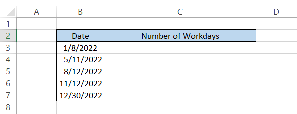
We will use the formula =NETWORKDAYS(DATE(YEAR(B3),1,1),B3) which gives the number of workdays between the two dates as:
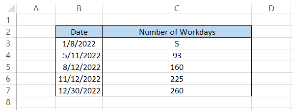
If we check the calendar, 1st January 2022, as well as 8th January both were Saturdays. The date from 3rd January to 7th January corresponds to Monday to Friday Work Days equalling five days which is precisely the result in cell C3.
Similarly, all the other workdays are also calculated similarly using the function.

Free Resources
To continue learning and advancing your career, check out these additional helpful WSO resources:


or Want to Sign up with your social account?