ERROR.TYPE Function
An Information Function that returns the integer that matches the value of a specific error.


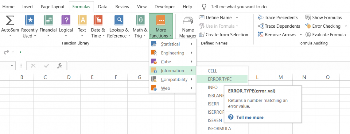
What is the ERROR.TYPE Function?
The ERROR.TYPE function in Excel is an Information Function that returns the integer that matches the value of a specific error. You can evaluate and test for different error values based on this function.
If Excel is your go-to application for financial analysis, brace yourself because you will deal with many formulas and functions while building models and making calculations in Excel.
However, sometimes wrong formulae can return errors throughout the Excel workbook. Manually identifying all the errors would probably take a lot of time. So what else can you do?
In this case, you can use the function. It will identify errors based on the number they return and may input other logical conditions based on the numbers corresponding to the errors.
In this article, we will explore what different errors you can encounter in Excel, their corresponding numerical value, and how to use this function to handle the errors.
- The ERROR.TYPE function is an Information Function in Excel that identifies the type of error that occurs in a cell.
- Users provide a reference to a cell containing an error as the argument to the ERROR.TYPE function. It returns a number that corresponds to the error type.
- ERROR.TYPE function helps users understand the nature of errors and take appropriate corrective actions, such as adjusting formulas, updating data sources, or refining data validation rules, to resolve errors and improve data quality.
- The function is commonly used in data analysis tasks, such as data validation, data cleaning, and error reporting, to identify and categorize errors within a dataset.
Understanding The ERROR.TYPE Function
The function is an information function that returns the number for a specific error value in Excel.
When you perform calculations in Excel, you will see a lot of different errors such as #N/A, #VALUE!, #REF!, #DIV/0, #NUM!, #NAME?, and #NULL! They indicate that whatever you are doing might be incorrect or the result returned might be invalid.
For example, Excel will usually return the #NAME? Error, when something needs to be corrected in the syntax or quotation marks are missing around the text string in the formula.
Similarly, when a formula such as VLOOKUP or HLOOKUP cannot find the value in a table, the function returns the #N/A error, which means not available.
When any of such errors, for example, #REF! is passed through the function, the result returned is number 4. If you have another #REF! Error, then Excel will return the same result.
We can conclude that each error will have a unique number assigned to it, and a similar error will give the exact number due to the function.
When you use the function, it displays the numbers for various errors that occur in Excel. The displayed list is just for reference, as Excel returns the unique number for you.
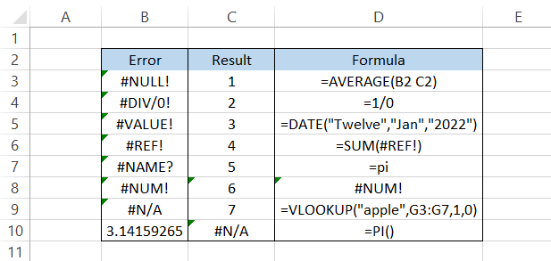
| Error_val | ERROR.TYPE result |
|---|---|
| #NULL! | 1 |
| #DIV/0! | 2 |
| #VALUE! | 3 |
| #REF! | 4 |
| #NAME? | 5 |
| #NUM! | 6 |
| #N/A! | 7 |
| #GETTING_DATA | 8 |
| #SPILL! | 9 |
| #CONNECT! | 10 |
| #BLOCKED! | 11 |
| #UNKNOWN! | 12 |
| #FIELD! | 13 |
| #CALC! | 14 |
Note
You will see some of the Error_val only in Excel 365.

types of errors in Excel
If we intend to understand how the function works, it is equally essential to understand the different errors in Excel. The mistakes and their specific numbers are
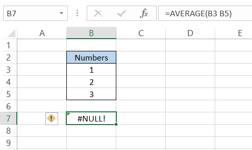
#NULL!
When a cell's range is incorrectly referenced or if you forget to use range operators such as colon(:) or comma(,) in the formula, Excel will return the exceptionally rare #NULL! error.
For example, if you are finding the average of the first three numbers using the AVERAGE function and forget to add the colon(:) between the starting and ending cell range, you will get the #NULL! error.
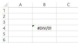
#DIV/0!
When you divide a number by zero, you will get the result as a #DIV/0 error. For example, try dividing 1 by 0 in Excel; you will get the result as #DIV/0.
#VALUE!
This type of error is returned when the values provided in the formula are of an unsupported type or, in general, when there is something wrong with the way the recipe is typed.
For example, because we unintentionally referenced cell C2 in our formula, which contains a text string, Excel returns the #VALUE! error.
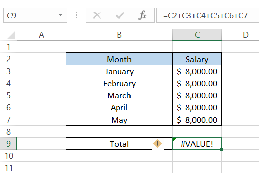
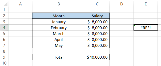
#REF!
These errors occur when you reference a particular cell or range of cells in a function that gets invalid either due to row/column getting deleted or when the formula gets copied to a new position where the reference becomes void.
For example, we have referenced five cells in our SUM formula used in cell C9. If you copy the formula in a cell less than five cells above the target cell, you will get the #REF! Error.
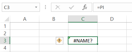
#NAME?
The #NAME? Error occurs when the quotation marks are missing around the text string in the formula, something needs to be corrected in the syntax(if the function is misspelled) or when Excel doesn't recognize something.
For example, if you use the PI function in Excel and forget to use the parenthesis, will you get the #NAME? Error.
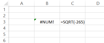
#NUM!
These errors usually occur when the number produced is either too big or too small, numerical calculations cannot be performed, or due to an invalid numeric value.
For example, if you try to take the square root of a negative number such as -265, using the formula =SQRT(-265), you will get the #NUM! Error.
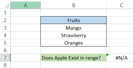
#N/A
#N/A Error occurs when Excel cannot find a value in a referenced range of cells. Suppose you use the VLOOKUP function to find 'Apple' among a range of fruits consisting of 'Mango',' Strawberry', and 'Oranges'; then you will get the #N/A error.
The error can be interpreted as the value not available in the referenced range. The formula used is =VLOOKUP("Apple", B2:B5,1,0), which gives the result as
#GETTING_DATA
The #GETTING_DATA Error is displayed by Excel when the workbook performs complex calculations that are not yet completed. It is a type of temporary error that cautions that user but usually disappears once the task in Excel is completed.
Another instance where you can see this error is when you import data from a CSV file with thousands of rows containing data.
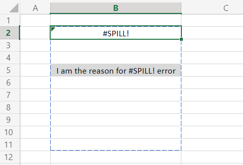
#SPILL! (Excel 365)
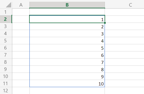
A #SPILL! Error occurs when the spilled ranges are blocked by non-blank cells in Excel. For example, we have used the SEQUENCE function in cell B2, such that the formula is =SEQUENCE(10,0,1,0).
Generally, the formula should give the result as illustrated below:
However, since we have a text value in cell B5, the 'spilled' values face resistance to flow into other cells. As a result, we get the #SPILL! error.
#CONNECT! (Excel 365)
Another transitory error occurs when you are trying to make connections in the workbook.
#BLOCKED! (Excel 365)
When the user cannot access a required resource, Excel returns the #BLOCKED! Error.
For example, if you are not authorized yet to try to establish external connections to other workbooks, then Excel returns the #BLOCKED! Error.
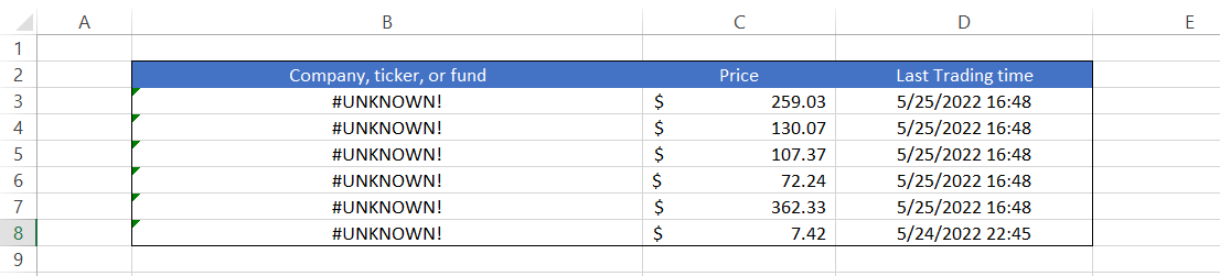
#UNKNOWN!
When an unsupported data type is used in Excel, it returns an #UNKNOWN! Error.
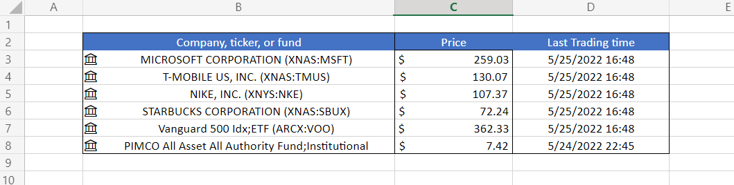
For example, we tried to import stock price and last trading time in Excel 365 using the Data tab, which gave the result as illustrated below:
However, when we tried running the same file in previous/older Excel versions, we got the #UNKNOWN! Error as earlier Excel versions did not support the data type.
#FIELD! (Excel 365)
When Excel is unable to find the referenced field in the linked data type, the error returned is #FIELD!
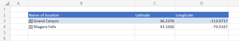
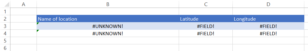
For example, we tried importing latitude and longitude for two different places Grand Canyon and Niagara Falls, using the 'Geography' function in Excel 365, which gave the result.
However, when we opened the same file in earlier Excel versions, we got the result as
#CALC! (Excel 365)
The CALC! Error occurs when the calculation mechanism used by Excel faces an undefined calculation error with an array.
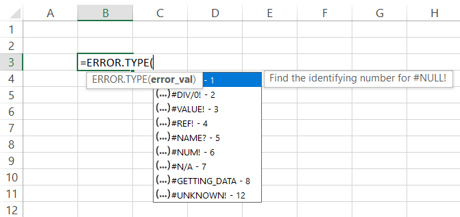
The syntax for the ERROR.TYPE function is:
= ERROR.TYPE(error_val)
Where error_val = reference to the cell that contains the error.

How to use the ERROR.TYPE Function in Excel?
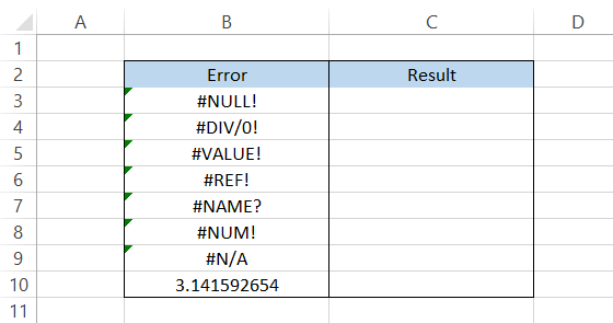
Assume that you have different errors in Excel, as illustrated below:
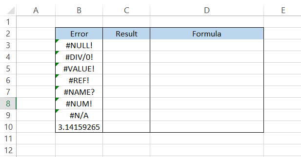
By using the formula
=ERROR.TYPE(B3)
in cell C3 and drag it down to cell C10. We will get the result as
If you might have noticed, when no error exists in our dataset, the function returns the #N/A! Error.
Practical Example
The ERROR.TYPE function alone might not have many practical applications, but combine it with the IF function, and you will have a process that handles all errors.
You must have wondered: Why does the function return numbers instead of resolving the error? The idea behind the process is to give users more flexibility to handle mistakes that would have been completely ignored.
We have several error-handling functions, such as IFERROR, IFNA, ISERR, and ISERROR. Still, they are limited in catering to either one particular error or all error types.
Assume that we have the errors in Excel as illustrated below:
Suppose there exist any #NULL! Error in our dataset, we want the IF function to return the result as "Syntax for the formula might be wrong" or else produce an empty cell.
For this, we will use the formula
=IF(ERROR.TYPE(B3)=1," Syntax for the procedure might be wrong," "),
which will give us the result as
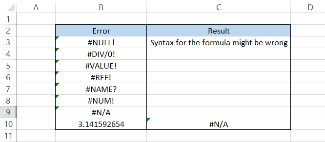
All the cells contain error returns as empty cells, except cell B10, which includes a value rather than an error. As the function evaluates the values to #N/A error; we get the same result in cell C10.
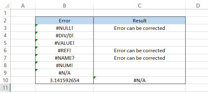
You can take it one step further by evaluating different errors to different values using nested IF or the IFS function.
By using the formula
=IFS(ERROR.TYPE(B3)=1,"Error can be corrected",ERROR.TYPE(B3)=4,"Error can be corrected",ERROR.TYPE(B3)=5,"Error can be corrected",TRUE,"")
you can evaluate the #NULL!, #REF!, and #NAME? errors in Excel and return a customized result while ignoring all the other errors in the process.
Free Resources
To continue learning and advancing your career, check out these additional helpful WSO resources:


or Want to Sign up with your social account?