COUNTIFS Function
A Statistical Excel Function that counts the Excel cells that match multiple specified criteria.


What is the COUNTIFS Function?
The COUNTIFS function is a Statistical Excel Function that counts the Excel cells that match multiple specified criteria.
The COUNTIF function also returns the cell count based on specified criteria. As both parts perform a similar task, they are often thought of as the same. But that's not the case.
The difference between them is that the COUNTIF will only accept one criterion, while its counterpart can buy more than one criterion.
The function uses different logical operators to input conditions which, if returned as TRUE for a particular cell, will increase the count for the final result.
Similarly, COUNTIF also allows wildcard characters to make a partial match for a text string and, if found, leads to an increase in the count for the result.
The function was introduced in Excel version 2007 and has since been present in all successive spreadsheet and analysis software versions.
This article will help you understand the syntax of the function, how to use the procedure, and how to best use financial and data analysis.
- The COUNTIFS function is a Statistical function that is used to count the number of cells that meet multiple criteria simultaneously.
- Users provide ranges and criteria pairs to the COUNTIFS function. It counts the number of cells that meet all the specified conditions.
- COUNTIFS function can be integrated into formulas and calculations to perform dynamic counting based on complex criteria or conditions, improving the efficiency and accuracy of data processing workflows.
- The function is commonly used in data analysis tasks, such as filtering and segmenting data based on specific criteria and calculating frequencies and distributions of categorical variables.
Understanding the COUNTIFS function
It is a statistical function that returns the cell count based on multiple predetermined conditions. If all the specified needs are met, i.e., the process evaluates to TRUE, then the value is counted as one for the range of selected cells.
Let's say you have demographic sales data for the North, South, East, and West regions. Each region has three cities, so you have data for 12 cities.
If you need to count the cells where the sales are more excellent than $8000 in 'City A' in the 'North' region, then you can input those criteria in the function, and it will return the result from thousands of the referenced cells.
The function iterates through all the cells and only counts those evaluated to TRUE for all the specified criteria.
It can count cells containing dates, numbers, text strings, and blank cells.
The function can be used for varied number-crunching tasks and data analysis by supporting wildcard characters and logical operators.
Excel users always argue that most functions are tricky to use and understand. But if the function falls under neither of those categories. So in the next section, we will see the syntax for the function.

COUNTIFS Function Formula
The syntax for the function is:
=COUNTIFS(criteria_range1,criteria1,[criteria_range2,criteria2]...)
Where
- criteria_range1 = (required) the first referenced range of cells that will be counted for the specified criterion
- Criteria = (required) the first condition that must be met to count the cells.
- criteria_range2 = (optional) the second referenced range of cells which will be counted for the specified criterion
- criteria2 = (optional) The second condition must be met to count the cells.
The function allows up to 127 pairs of range/criteria for counting cells based on predetermined conditions.
To make the function more efficient, there are two additional components that you can use to get better results in Excel. They are logical operators and wildcard characters.
Logical Operators
The logical operators play an essential role in specifying different criteria in the function. In addition, these comparison operators help to compare numbers, strings, and dates and perform complex assessments of the conditions.
Listed below are the logical operators that you can use while using the function:
| Condition | Operator | Description |
|---|---|---|
| Equal to | = | Compares two values and returns TRUE if they are equal, |
| Not equal to | <> | Compares two values and returns TRUE if they are not equal |
| Greater than | > | If one value is greater than the other, then the condition evaluates to TRUE. |
| Less than | < | If one value is less than the other, then the condition evaluates to TRUE |
| Greater than or equal to | >= | The condition returns as TRUE if the value is greater than or equal to another value. |
| Less than or equal to | <= | The condition returns as TRUE if the value is less than or equal to another value. |
The logical operators improve the versatility and efficiency of the function; it is not essential to use them while specifying the criteria. It is entirely up to you whether you use them or not.
Wildcard Characters
Wildcards are special characters that return results by substituting them with other characters. With wildcards, you can make partial matches among a range of cells and count the cells that match your substring + wildcard character.
One of the most used wildcard characters is the apostrophe(*), which matches the substring before the wildcard and returns all the strings that might fit that combination.
For example, if you need to find all the files that begin with a substring. Exc*, all the potential files could be Excel_1, Excel1, Excelllllllllll_1, etc.
The only requirement is that the first three characters are the same, while the rest could be anything that matches all the available options.
There are several wildcard characters that you can use, each of which functions differently with a supplied text substring. Some wildcards are:
| Characters | Explanations | Examples |
|---|---|---|
| * | It matches the characters before * with text and returns all the strings. | he* will return hello, hell, hebrew but not chef, chew. It would have returned the latter words for che* |
| ? | It will match a single alphabet position of a text string. | bee? Will return beer, beep, beet, etc |
| [] | It will match characters within the square brackets | bee[rt] will return beer, beet but not been |
| [ ] + ! | An exclamation mark followed by characters inside brackets excludes them from the text match | bee[!rt] will not return beer, beet but will return beep, been |
| [ ] + - | A range of alphabets(in ascending order) separated by a dash in brackets matches all the similar text in the string | a[a-c]c will return aac, abc, acc |
| # | It will match numerical characters. | 2#2 will return 252, 212, 222. |
How to use the COUNTIFS Function?
The function can be used in two different ways. You can choose either method at your convenience because, ultimately, you will get the same result.
Method 1: From the function's library
Functions are the pre-established formulas where you just input the arguments and directly get the result in the selected cell. For example, to use the function, please follow the steps below:
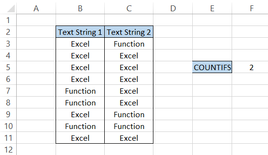
- First, select the cell count for the result based on multiple criteria:
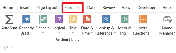
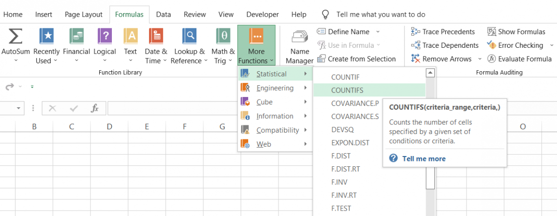
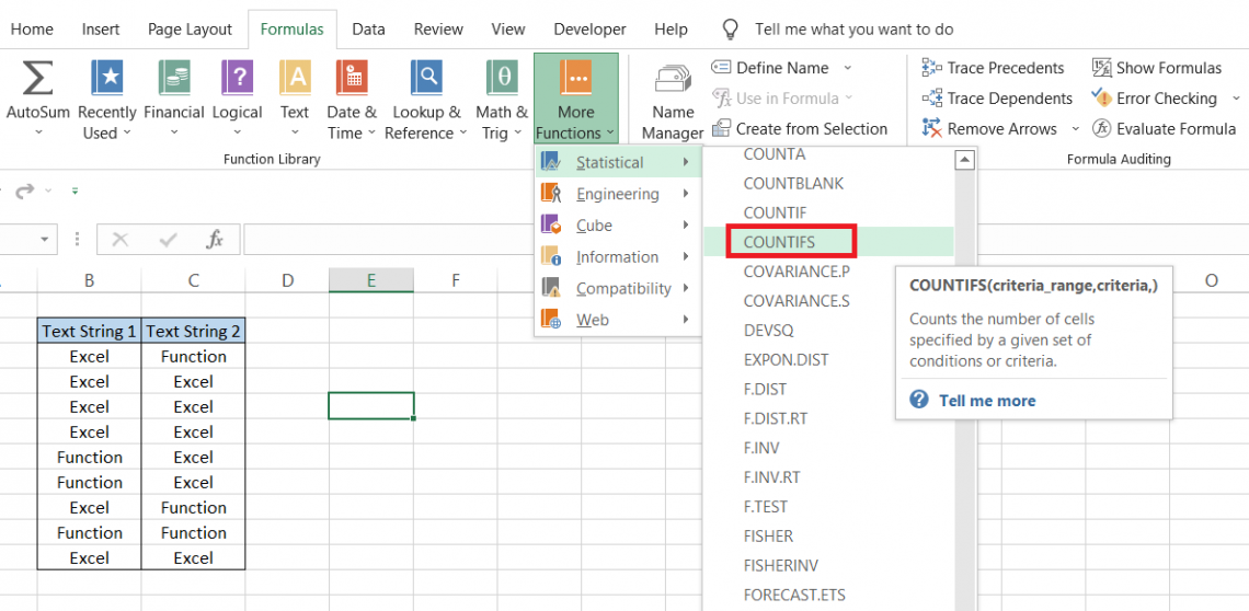
- Next, click on the Formulas tab > More Functions > Statistical and then search for the COUNTIFS function and click on it:
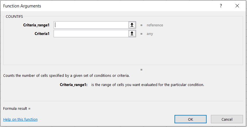
- This will open up the dialog box as illustrated below:
- In a range of cells consisting of the text string' Excel,' we are trying to find the string 'Function' as our criteria while the second criteria are precisely the opposite.
In short, the formula will only count those cells that evaluate TRUE for 'Function' in range_1 and 'Excel' in range_2.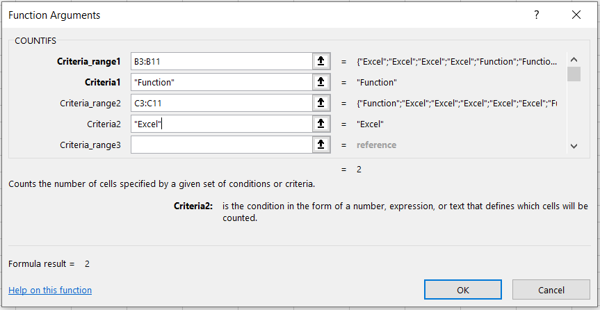
- Even before clicking on Ok, we get a preview of what our result would be in the dialog box, as illustrated below:
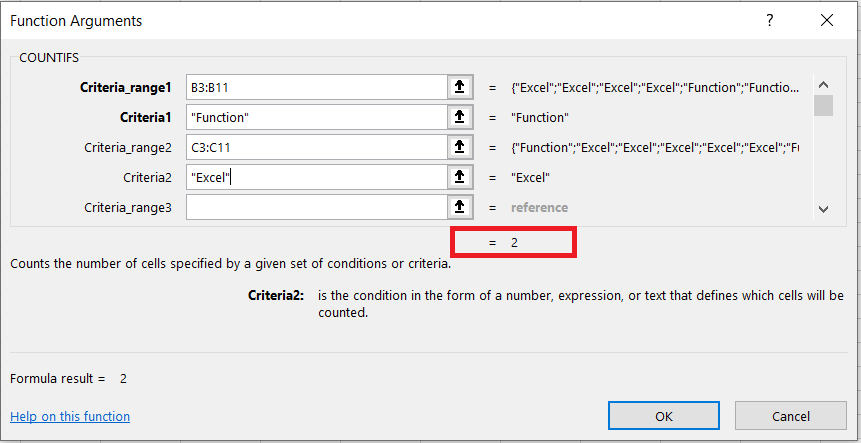
- When you click on Ok, you will get the result as 2 in the selected cell:
Method 2: As a worksheet function
To use the function as a worksheet formula, you begin with an equal sign and input the function name followed by the arguments in the function.
Suppose that you need to count on how many instances the sales in the 'North' region are greater than $500.
The data looks as illustrated below:
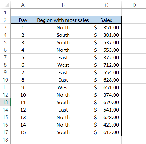
To find the cell count, we will use the formula
=COUNTIFS(B3:B17, "North", C3:C17, ">500"),
which will give us the result as 2.
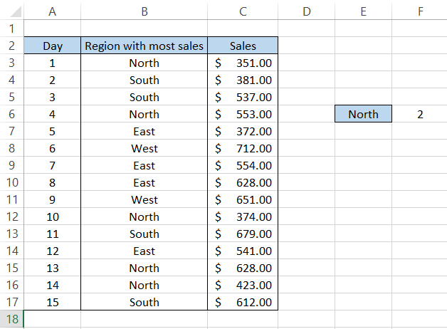
On closer inspection, we find that the 'sales' in cells C6 and C15 are the only values with a North region with sales greater than $500.
Our final result ignores all sales below $500 for the North region.

COUNTIFS Function Examples
The function was introduced as a successor to COUNTIF since the latter could accept only one criterion.
The scenario for financial and data analysis was changing fast. The option to use a combination of logical functions to input multiple conditions was available, but it wasn't feasible for every Excel user in the community.
Microsoft thought a change was necessary, and they delivered it in the form of COUNTIFS in 2007, which accepted multiple criteria along with wildcard characters and logical operators.
In the consecutive sections, we will see a couple of examples to help us understand the function even better.
Example 1: Counting based on Text strings
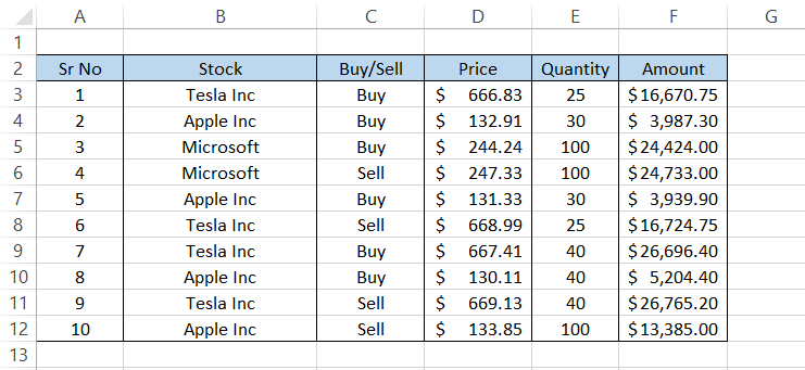
Today was a good day for you as a day trader. You made $685.20 from various intraday positions, and your faith is slowly building that you can outperform all the hedge fund managers.
But, at the end comes the critical part - Assessing all the positions taken for the day. The data looks as illustrated below:
To find the count for all the 'Tesla' buy trades with a quantity greater than 25, we will use the formula
=COUNTIFS(B3:B12, "Tesla Inc," C3:C12, "Buy," E3:E12, ">25"),
which should give you the result as 1.
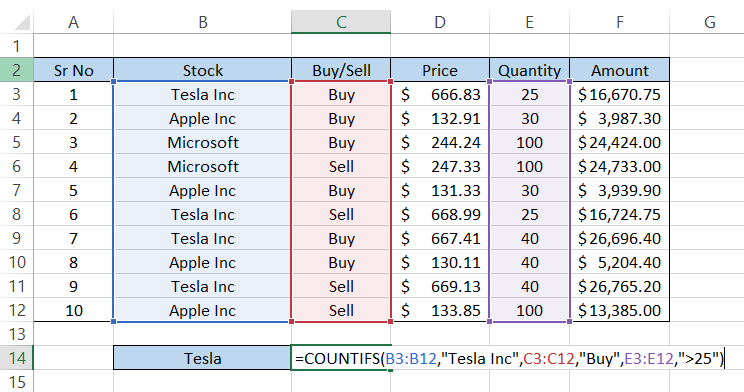
In this example, we specified three different criteria, i.e.,
- Filter out Tesla Inc
- Buy signals
- Only the trades with a quantity greater than 25(Not even equal to 25!).
The function iterated through all the cells in the background, making imaginary checks, and finally found that row 10 satisfied all the conditions and, thus, gave the result as 1.
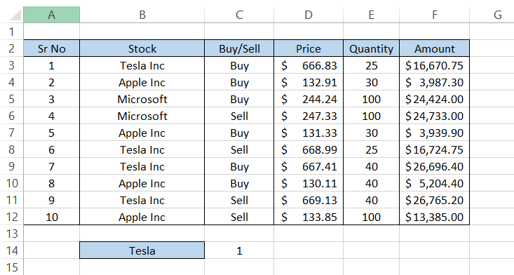
Since you know what formula to use, you can substitute the other values and find their respective counts!
Example 2: Counting based on cell references and logical operators
Let's just agree that hardcoding the criteria is really an efficient method in the long run. You wouldn't want to update the formula on every instance when the underlying assumptions in your Excel model change.
Rather you can just input the value in a cell and then reference it into the formula. Now, even if the underlying value changes, you just need to update the cell value, not the formula.
For example, suppose you work at a financial company that offers loans to other businesses and individuals. For companies that take loans to provide loans to other people further, the delinquency rate must not be greater than 4.15%.
The delinquency rate refers to the percentage of loans in a company's portfolio where the borrowers are not paying their installments on the due date.
The other parameter that the company must adhere to is its delinquency rate. Since they have borrowed money from you, they intend to pay you the installments, where the delinquency rate must not exceed 2.5%.
The data looks as illustrated below:
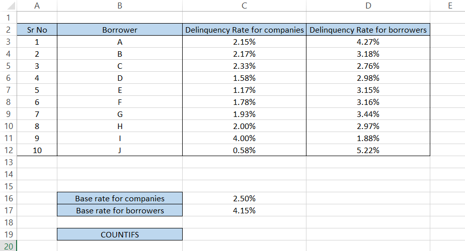
To count the cells that fulfill both criteria, we will use the formula
=COUNTIFS(C3:C12,">" &C16,D3:D12,">"Which),
which will give us the result:
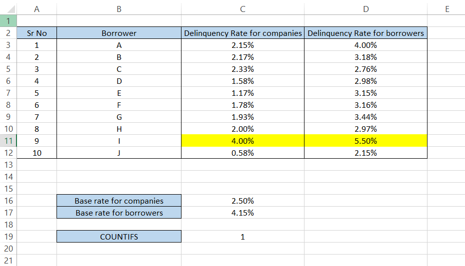
Only on one occasion did both criteria evaluate TRUE, which provides us with the count of cells as 1. Now, if the base rate for both companies and borrowers was changed, you can just input the values in cells C16 and the C17; the formula would do the rest!
The company lending money to other borrowers would fail to pay installments to your financial institution since they cannot receive any payments from their borrowers.
In such a case, the financial institution can have two choices - reduce the total amount of money lent, i.e., if they were previously willing to lend 90% of the collateral, now they would lend only 80 or 70%.
The other option is to claim the collateral from the joint account, but that rarely happens unless the borrowing company cannot pay a single dime.
Example 3: Counting based on wildcards
If you have read the example about wildcards in our COUNTIF function article, you already know what we are speaking about.
If it weren't for the wildcard characters, our life as Excel users would have been much more difficult.
Suppose your sales for the stationary supplies are as illustrated below:
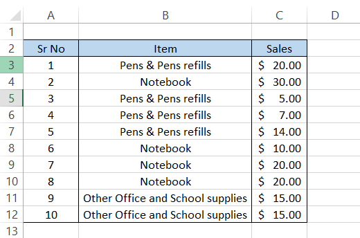
You can find the count of all the cells where sales for 'Pens & Pens refills' was more than
$12 with just the substring' Pen.'
By using the formula
=COUNTIFS(B3:B12,"Pen*",C3:C12,">12"),
we should get the cell count as equal to 2.
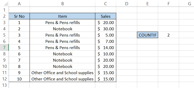
Even after using just a substring of our entire text string, the function could identify all the relevant text strings and return their count in cell F5 as 2. The other substrings you would have instead used are 'pens refills' or just 'refills.'
The substrings must be unique to find the original text string, or else there is a high probability the formula may return a false positive result.
The use of wildcard characters takes the flexibility of the function up to a whole new level.
Example 4: COUNTIFS with array constants
When the number of text string criteria is more, adding them as arguments can be quite a hassle as it would make your formula far more complicated.
In such a case, you can input the text strings as an array and get the count using the COUNTIFS and SUM functions.
Suppose that the data looks as illustrated below:
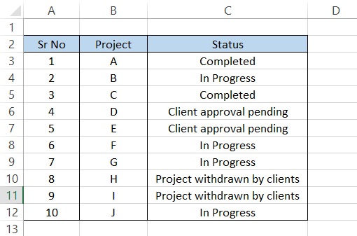
Of all the four text strings, we would like to evaluate all as criteria except 'Completed.'
Therefore, we will use the formula:
=SUM(COUNTIFS(C3:C12,{"In Progress","Client approval pending","Project withdrawn by clients"})),
which will give us a result of 8.

Whenever the status is equal to 'In Progress,' 'Client approval pending,' or 'Project withdrawn by clients,' the formula calculates the value as one. Finally, it returns a cumulative result that is equal to eight.
Similarly, you can input multiple text criteria that would only return the count when all the requirements evaluate to TRUE.
Example 5: Finding the count between two numbers.
By now, you should understand that the formula can include multiple criteria and that logical operators improve the function's flexibility.
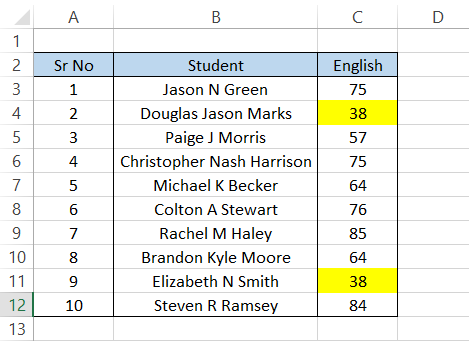
Suppose that you intend to find how many students have scored marks between 35 and 50. Then, we can combine both the components of the function and return the result based on the evaluation.
The data for the marks scored by students looks as illustrated below:
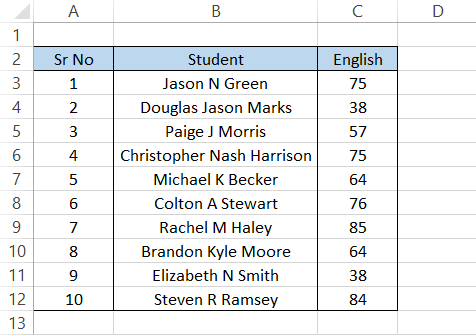
To find the cells with marks between 35 and 50, we will use the formula
=COUNTIFS(C3:C12, ">35", C3:C12," <50"),
which will give you the result as illustrated below:
Only two students scored marks between 35 and 50 in the English subject.
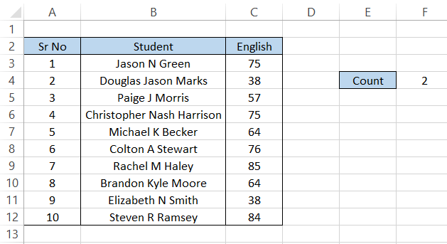
Let's say we want to highlight the cells based on the COUNTIFS result. To seek help, we turn to the Conditional Formatting tool.
Select the range of cells, i.e., C3:C12, click on the conditional formatting tool from the Home tab, and set a 'New Rule' from the drop-down menu. This will open up the dialog box where you will input the formula.
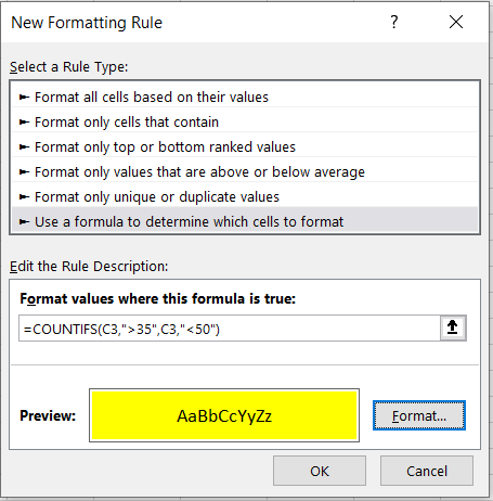
Once you click on Ok, the formula will iterate through all the cells and highlight those cells that evaluate the results for the TRUE condition.
You will get the result as illustrated below:
If you thoroughly explore the potential of both COUNTIFS and the conditional formatting function, no one can stop you from becoming an Excel wizard!
Free Resources
To continue learning and advancing your career, check out these additional helpful WSO resources:


or Want to Sign up with your social account?