AVERAGE Function
An Excel Statistical function that calculates the arithmetic mean of given observations, a range, or a data set.


How to Calculate AVERAGE in Excel?
The AVERAGE function is an Excel Statistical function that calculates the arithmetic mean of given observations, a range, or a data set. The primary use of the AVERAGE function is to assess the average value of the data.
The AVERAGE function calculates the arithmetic mean by summing the given observation and dividing it by the number of observations.
The AVERAGE function in Excel finds the average of the supplied series of numbers.
Finding the average for numbers was one of childhood's most common arithmetic calculations. But, unfortunately, the standard was often interchanged with another mathematical concept: the mean.
When asked to find the average or mean of a series of numbers, we add all the numbers and then divide the result by the total number of values.
For example, if we have five numbers and get their total as 40, the average of the numbers will be equal to 8, i.e., 40 divided by 5.
The calculations seem simple when we have a few numbers, but what if you have hundreds of rows of data?
Maybe, in that case, you could use the SUM and COUNT functions in the numerator and denominator, respectively, but why go through all that trouble when you could get the same result using a single position?
In this article, we will understand the syntax for the function, how you can use it, and a couple of examples to help you understand the function better.
- The AVERAGE function in Excel is a statistical function used to calculate the average (arithmetic mean) of a range of numbers. It is also used to find a dataset's central tendency.
- The syntax for the AVERAGE function includes one argument: number1 (required), which is the first number or range for which you want the average.
- The AVERAGE function is commonly used in financial modeling, scientific data analysis, and everyday calculations to find the average of a dataset. It is helpful for summarizing data and finding typical values.
- The AVERAGE function ignores non-numeric values and empty cells in its calculation. If all the arguments are non-numeric or empty, it returns a #DIV/0! error.
Understanding AVERAGE function
The AVERAGE is categorized as a Statistical function that finds the average for a range of values.
For example, suppose you have three numbers: 5, 8, and 13. If you use the function to calculate the average, you will get 8.67.
What exactly goes behind the scenes? The three numbers are first added together using the simple arithmetic expression, which gives the result of 26. The result is then divided by 3, which is our example's total number of observations.
When you divide 26 by 3, you will get the result of 8.67. The calculations are as illustrated below:
= (5 + 8 + 13)/3
= 26/3
= 8.666666667
When you use the function in Excel, you can either hardcode the numbers directly in the formula, the reference range of cells, or even reference a procedure that returns a numerical value.
The function can accept numerical values, whatever the source may be, but some of the things that the part ignores are blank cells, text strings, and boolean values.
Next, we will see what the syntax for the function is.
The syntax for the function:
=AVERAGE(number1,[number2]...)
Where,
- number1 = (required) number, cell reference to a numerical value or a formula that returns a number
- number2 = (optional) number, cell reference to a numerical value or a formula that returns a number.
You can input up to 255 optional arguments in the function as hardcoded values or cell references.
How to use the Average function?
If you are to use the AVERAGE function in Excel, there are two different methods.
Method #1: From the function's library
To use the AVERAGE function from the library, please follow the steps below:
- Select the cell in which you intend to get the result.
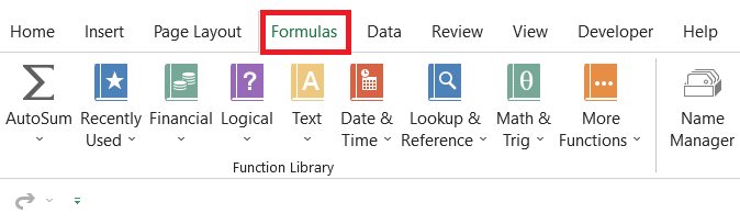
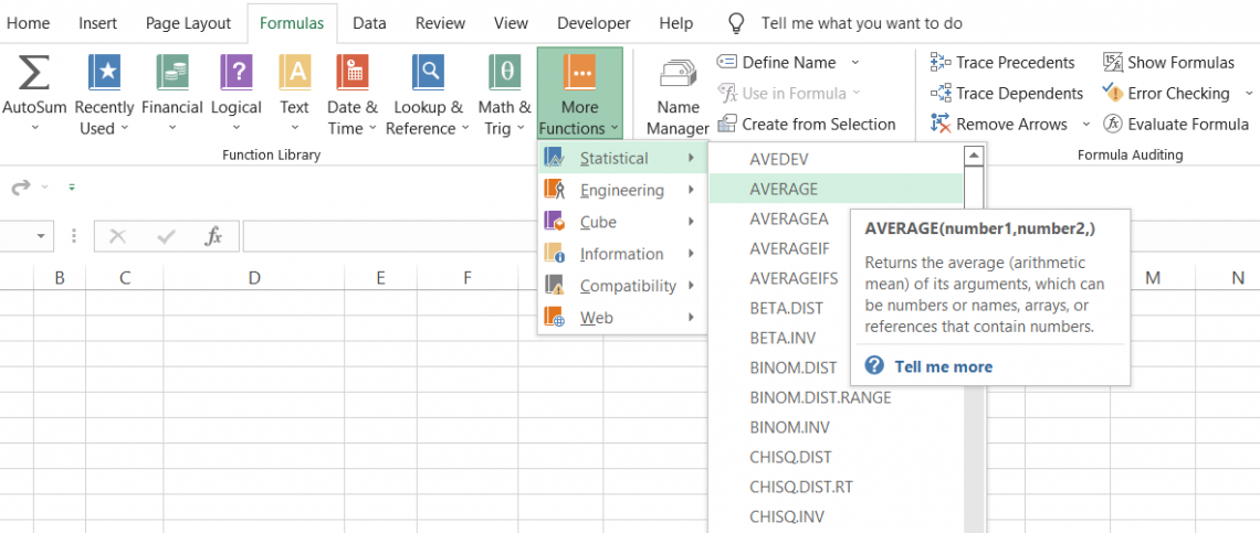
- Click on Formulas tab > More Functions > Statistical > select the AVERAGE function.
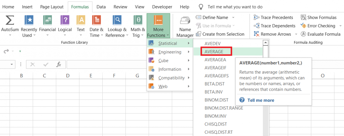
- This should open up the dialog box, as illustrated below:
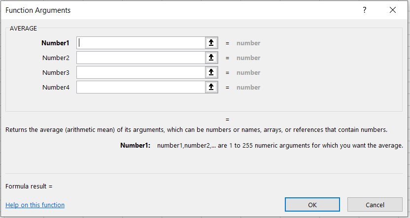
- Here, we will input the arguments in the function as per the syntax. For example, suppose we input three numbers, 5, 8, and 13, in the dialog box as:
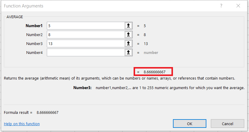
- Based on the inputs, we get a preview of what the expected result would be, which is equal to 8.666666667
- Once you click on Ok, you will get the same effect in the selected cell.
Method #2: As a Worksheet formula
Using the function as a worksheet formula is the most popular method used by Excel users. The worksheet formula offers greater versatility to combine different functions and improve efficiency while working in Excel.
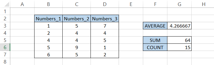
Suppose that you have the data as illustrated below:
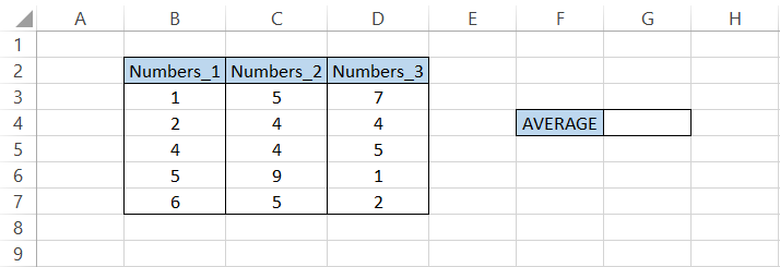
We need to find the average of all the numbers in columns B, C, and D, respectively.
To get the mean value in cell G4, we will use the formula =AVERAGE(B3:B7, C3:C7, D3:D7), which gives the result:
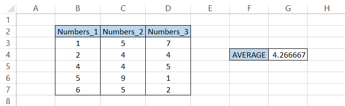
The function makes calculating the mean value accessible by referencing the cell or range of cells in the process.
If the function did not exist, what could have been the alternative?
We discussed how you could use the combination of SUM and COUNT functions to get a similar result. But, first, we will use the SUM function to get the total of all the numbers in column B, column C, and column D.
The formula will be =SUM(B3:B7, C3:C7, D3:D7), which gives us the result of 64.
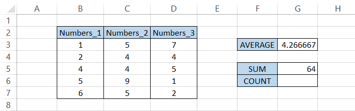
Next, we will use the COUNT function using the formula =COUNT(B3:B7, C3:C7, D3:D7), which gives the result in cell G6 as:
When you divide SUM by COUNT, the result is the same as the AVERAGE function.
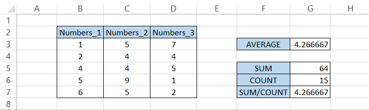
Excel saves us from wasting time in all these calculations by directly allowing us to reference the cell and return the mean value.
Example of the AVERAGE function
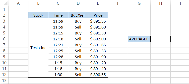
Suppose that you day trade for a living. You make a series of works in Tesla Inc. and need to determine the average traded price for the stock.
The data looks as illustrated below:
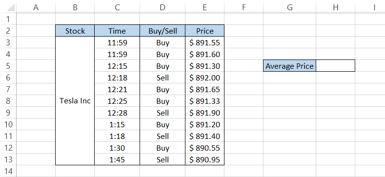
Here, we will ignore whether the transaction was a 'buy' or 'sell.' Our intention is only to find the mean price.
To get the mean value, we will use the formula =AVERAGE(E3:E13) in cell H5, which gives the result:
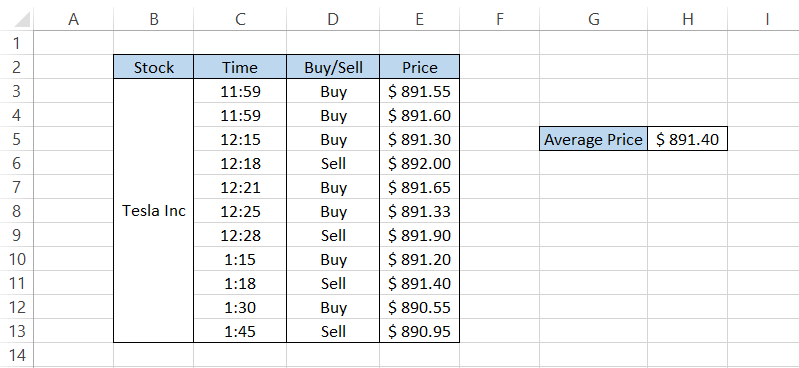
The average traded price for Tesla Inc. is $891.40 based on all the transactions. What if you wanted to determine the mean price for the 'buy' transactions?
You all are brilliant. We believe the first function that came to your mind is the AVERAGEIF, i.e., if a condition is fulfilled, then return the mean value. However, what if the AVERAGEIF function did not exist?
Scary thought, but we do need a solution to the problem. Here, you can use the combination of ISNUMBER, MATCH, and AVERAGE functions.
To get the mean price for 'buy' transactions, we will use the formula, =AVERAGE(IF(ISNUMBER(MATCH(D3:D13,{"Buy"},0)), E3:E13)), which gives us the result as:
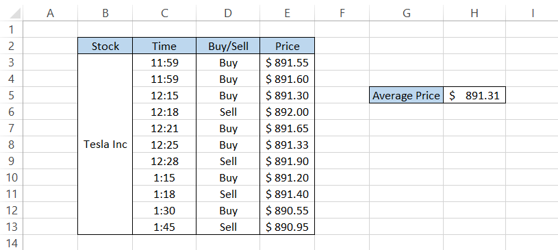
The average price you paid for all the 'buy' transactions is $891.31, as illustrated in cell H5. Since this is an array formula, you need to press Ctrl + Shift + Enter after you input the procedure in the cell.
How does the formula work?
The following are the ways the the AVERAGE function works.
- Firstly, the MATCH function finds all the 'buy' transactions in the range D3:D13. Since we have set the match_type to match, the function returns TRUE if the value is found and #N/A Error if the value is missing.
- Based on this, you would get the array as {TRUE, TRUE, TRUE, #N/A, TRUE, TRUE, #N/A, TRUE, #N/A, TRUE, #N/A}.
- The ISNUMBER function checks whether the referenced value is a number or not. The boolean value TRUE equals 1, while FALSE equals 0. When you pass the array through ISNUMBER, the formula will return another array {TRUE,TRUE,TRUE,FALSE,TRUE,TRUE,FALSE,TRUE,FALSE,TRUE,FALSE}.
- Based on this final array, the IF and AVERAGE function works together to find the mean for TRUE values from the collection in the corresponding range E3:E13.
NOTE
Since this is an array formula, you need to press Ctrl + Shift + Enter after you input the procedure in the cell.
AVERAGE vs. AVERAGEA
You might have discovered another function that might look like a counterpart to the article's hero. The process in question is none other than - AVERAGEA.
On closer inspection, we find that there is absolutely no difference in the function name apart from the 'A' at the end. So how does that make it different?
The most significant difference between the two functions is that AVERAGEA also evaluates boolean values, such as TRUE and FALSE, and text strings in the formula.
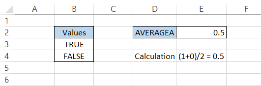
We know that TRUE is stored as 1, while FALSE is stored as 0 in Excel. Therefore, when you reference a cell consisting of both values and use the AVERAGEA function, you will get a result of 0.5.
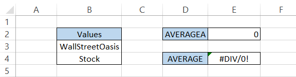
Similar to FALSE, the text strings as well are stored as 0. If you reference a couple of text strings in the formula, you will ultimately get the result of 0.
However, it is not the same case with the AVERAGE function. You would only get the #DIV/0! Error if you reference text strings in the formula.
Now, the big question remains: What is the function's syntax?
The syntax for the AVERAGEA function is:
=AVERAGEA(value1,[value2]...)
Where,
- value1 = (required) the boolean value, i.e., TRUE or FALSE, text string, numerical value, or reference to cells containing any of those values.
- value2 = (optional) the boolean value, i.e., TRUE or FALSE, text string, numerical value, or reference to cells containing any of those values.
You can input up to 255 arguments in the function as a hardcoded value or as a cell reference.
Suppose that you have the data as illustrated below:
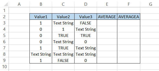
First, we will find the mean value of the range B3:D3 in cell E3. Then, we will use the formula =AVERAGE(B3:D3), which gives the result:
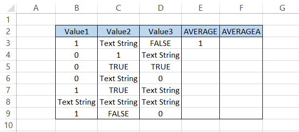
Even though text strings and boolean values exist in the range, we still get the mean value since a numerical value exists. All the other unwanted values get ignored.
Now drag down the formula up to cell E9, which gives the result:
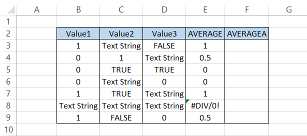
In the range B8:D8, we see that all the values are text strings, so the result we get is #DIV/0! Error.
On the other hand, by using the formula =AVERAGEA(B3:D3) in cell F3 and dragging it down, we get the result:
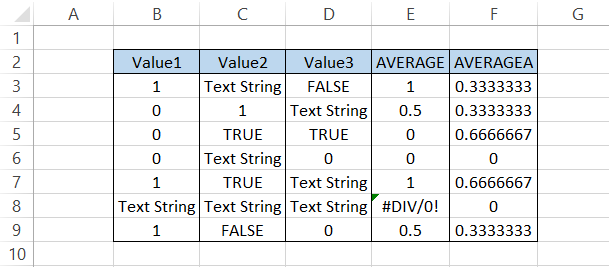
If we have a non-empty cell, it will be counted as a value in finding the mean value. Only if the cell is empty will it be ignored from the result. The calculation of the mean value for range B3:D3 is, as illustrated below:
= (1 + Text String (0) + FALSE (0)) / 3
= (1 + 0 + 0) / 3
= 1/3
= 0.333333
This way, you can also calculate and recheck whether the results obtained in column F are accurate.

AVERAGE vs. AVERAGEIF
Another critical function that you must know about is the AVERAGEIF function. Perhaps we talked about it in one of the earlier examples.
The function finds the mean value based on the criteria you input. If the classic matches, Excel finds the mean value of all the requirements passing cells.
The syntax for the AVERAGEIF function is:
=AVERAGEIF(range,criteria,[average_range])
Where,
- range = (required) the field of cells that will be checked for the criteria. The content may include text strings, numbers, arrays, or results derived from formulas.
- criteria = (required) the condition based on which the cells will be averaged. It may include text strings, numbers, or cell references. For example, 'buy', '>126,' etc.
average_range = (optional) the range of cells that will be averaged. The range is considered for calculating the mean value if the argument is omitted.
Let's see a quick example to understand how the function works. First, suppose that you have the data as illustrated below:
If you want to find the mean price for all the 'Sell' transactions, we will use the formula, =AVERAGEIF(D3:D12, "Sell", E3:E12), which gives us the result:
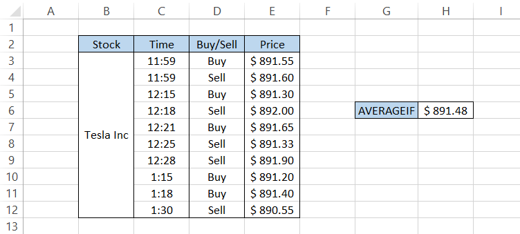
If we add up all the 'Sell' transactions and divide the total number of values, we will get the same result, which is $891.48.

Free Resources
To continue learning and advancing your career, check out these additional helpful WSO resources:


or Want to Sign up with your social account?