CHISQ.INV.RT Function
Displays the inverse of the right-tailed chi-squared distribution function for a specific set of data.

What is the CHISQ.INV.RT Function?
The CHISQ.INV.RT function in Excel displays the inverse of the right-tailed chi-squared distribution function for a specific set of data.
So, the CHISQ.INV.RT function is the inverse of the Chisq Dist Rt function, which is the continuous probability distribution. This distribution computes the probability of reaching up to or less than a specific value for a chi-squared statistic.
The chi-squared test generates its respective statistic. This forms a crucial part of statistics and hypothesis testing.
This is done to study whether two or more variables are independent of each other in influencing a particular outcome or dependent variable. So, it examines the degree of independence of the variables at hand.
CHISQ.INV.RT Function = CHISQ.INV.RT(probability,deg_freedom) or CHISQ.INV.RT(x,deg_freedom)
In the Excel formula, there are two components, which are:
- X: the observed value and probability: the probability for the chi-squared distribution with this set of data and parameters
- Deg_freedom: the number of degrees of freedom for the particular data being studied
Note
The CHISQ.INV.RT function also incorporates an iterative search technique, which performs repetitive search tasks. If the search does not converge after completing 64 iterations, the Excel spreadsheet will showcase a “#N/A” error value.
- The CHISQ.INV.RT function is a statistical function in Excel used to calculate the inverse of the right-tailed chi-square distribution, which is commonly used in hypothesis testing and confidence interval construction.
- The first two instances when the CHISQ.INV.RT function should not be performed when the chi-squared statistic appears as a negative number or greater than the critical value required.
- The third instance is when the value for degrees of freedom is less than or equal to 1.
- #VALUE! And #NUM! error values can arise when errors in inputting the values occur, such as entering non-numeric values or values that do not fall within the required range for the probability and degrees of freedom.
Understanding The CHISQ.INV.RT Function
Based on a particular probability value, the Chisq Inv Rt function tries to find the value x so that the value of the Chisq Dist Rt function (given x and a particular number of degrees of freedom) is equal to the probability.
So, the function and its precision in delivering results are based on the precision of the distribution function.
After attempting to execute the Chisq Inv Rt function in Excel, several cases can occur, influencing the results based on probability and degrees of freedom.
This is outlined clearly in the following points:
- If either the probability or degrees of freedom is entered as a non-numeric value, CHISQ.INV.RT will show the #VALUE! Error value
- If the probability is less than 0 or greater than 1, the CHISQ.INV.RT function will reveal the #NUM! Error value
- If the input for deg_freedom is not an integer, the value is truncated, meaning it is shortened by limiting the number of digits to the right of the decimal point
- If the input for deg_freedom is less than 1, the CHISQ.INV.RT function will show the #NUM! Error value
As useful as possible, there are three circumstances when individuals should avoid using the Chisq Inv Rt function. These are as follows:
- If the data contains a negative number for the chi-squared statistic
- If the quantity for degrees of freedom is less than or equal to 1
- If the chi-squared statistic in a particular data set is greater than the critical value for the significance level under consideration

How to use the CHISQ.INV.RT Function in Excel?
Suppose we have a data set with the below values for probabilities and degrees of freedom.
| Probability | Deg_freedom |
|---|---|
| 0.1 | 10 |
| 0.25 | 12 |
| 0.25 | 2 |
| 0.25 | 3 |
| 0.65 | 5 |
| 0.65 | 12 |
To calculate the inverse of the one-tailed probability of the chi-squared distribution, we must enter the formula “CHISQ.INV.RT” and select the relevant cells before clicking the Enter key. This would generate something like the following results in the Excel spreadsheet:
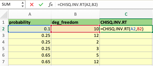
The formula would be typed out as “=CHISQ.INV.RT( without a space before the equal sign), after which the relevant cells for probability and degrees of freedom can be selected, or the cell numbers can be typed out with a comma separating the two values.
Afterward, the parentheses opened before selecting the cells must be closed. Now, the function is ready, and hitting the Enter key showcases the Chisq Inv Rt function's result for the selected values.
The formula is in cell C2 and typed out in the fx box above the rows and columns, which displays the function being executed at this particular time.
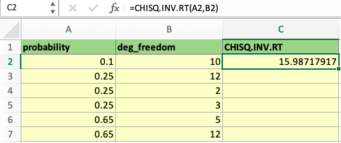
So, in the highlighted cells of the second row, the CHISQ.INV.RT function command generates the result by incorporating a probability of 0.1 from cell A2 and 10 degrees of freedom from cell B2.
This is shown in the screenshot below in the green highlighted text box, cell C2:
From there, we can apply the same formula to the following values in rows 3-7 or any set of values for the probability and degrees of freedom. This can be done manually by typing the formula again in the boxes below C2 or clicking on the AutoFill Handle and dragging it down.
To activate the AutoFill Handle option, we start by clicking on the square in the bottom right corner of the highlighted cell, C2, and dragging it down to cover cells C3 to C7. This is shown below:
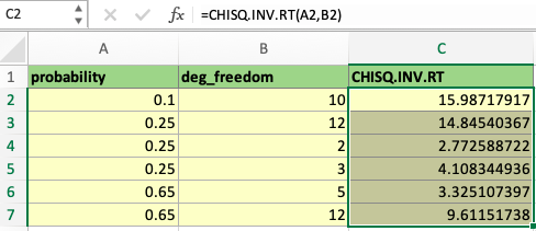
By doing so, the Chisq Inv Rt function has been applied to the other sets of probabilities and degrees of freedom, and so it is a quicker way of applying the same formula. This is useful when handling long rows and large amounts of data in a single study.
Therefore, the Chisq Inv Rt function allows us to calculate the inverse of the chi-squared distribution function. Then, we can use those values to conclude the relationships between the probabilities, degrees of freedom, and the function results in a specific data set.
For example, as the number of degrees of freedom increases (from B4 to B5 or B3), the result of the Chisq Inv Rt function increases, looking at the respective cells in column C. However, as the probability increases (comparing A3 and A7), the function's result decreases.
With more opportunities that the value had to be large (degrees of freedom), the critical value must be more significant to have data above the noise level.

Free Resources
To continue learning and advancing your career, check out these additional helpful WSO resources:


or Want to Sign up with your social account?