CONFIDENCE.NORM Function

A confidence interval is an estimation of the range of values within which a population parameter falls.

It shows the preciseness of an estimate for parameters such as the mean, and this is typically taken from a sample of the population.

The rationale behind this method is straightforward. It is incredibly difficult to analyze each population observation; hence one can only make an informed deduction on what the mean and variance can be for a vast dataset.

This is where sampling comes in; population parameter estimates such as the mean or variance can be calculated using a sample of the overall population.

For example, if the heights of 100 women are recorded in Boston, the results of this sample might provide insights into the mean height for every woman in Boston.

A confidence interval simply measures how accurately a sample represents its population. The probability that the true mean value of a population is included within the confidence interval range is referred to as the confidence level.

For instance, a confidence interval with a 95% confidence level implies that there is a 95% chance that the population’s true mean falls between the upper and lower bound estimates of the confidence interval.

Any continuous data variable will follow a normal distribution. If a specific scenario is run an infinite number of times, mapping each occurrence will return a bell-shaped histogram where the values are symmetric around the mean. 

Therefore, visually plotting a population can confirm whether the data follows a normal distribution. Once this is checked, a population sample can compute confidence interval estimations.

Confidence intervals are dependent on the underlying assumptions of the central limit theorem (CLT). CLT states that as you increase the number of observations, the distribution of said observations will increasingly resemble a normal distribution. 

The Confidence Normal Distribution

Also known as gaussian distribution, normal distribution describes how a set of data is spread around its mean. It results in a symmetrical distribution which takes the shape of a bell curve; data points away from the mean are fewer in number and at extreme ends.

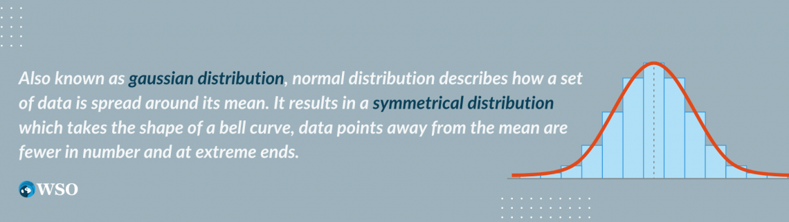
The premise behind this is that if one samples an event an infinite number of times, then the data spread will mimic a bell shape where most instances are concentrated around the average.

It has various real-world applications, as height, weight, or IQ can be modeled using normal distribution. Additionally, it can be well-defined mathematically, making it an ideal tool to work with for statistical analysis.

If a sample is normally distributed, the standard deviation and similar statistical properties can be estimated with more accuracy. This leads to better-defined confidence intervals too.

Normal distribution is the foundation for various statistical concepts such as hypothesis testing, linear regression, and confidence intervals; its intuitive nature makes it the single most important phenomenon in statistics.

Normal distribution is the bedrock on which confidence intervals are built. Without the continuous probability distribution created by the bell curve, it would be difficult to say, with confidence, how precise a range of estimates for a certain population parameter is. 

Confidence Interval Components & Formula

To understand the confidence interval formula, one must first define a z-score. The z-score is a standardized value that defines how many standard deviations away a certain observation is from the mean.

This is imperative in comparing data from different distributions. A positive z-score of +1 would mean the data point in question is one standard deviation above the mean. In comparison, a negative z-score of -1 represents an observation that is one standard deviation below the mean.

A z-score of 0 suggests that the sample value exactly falls on the population's true mean. This is a rare occurrence. Similarly, a z-score higher than +1.96 or lower than -1.96 can be considered a statistically significant outlier.

Where 

•  x: a single observation from the sample of the population
•  μ: mean of the entire population
•  σ: Standard Deviation of the population 

Once a z-score has been found, one can refer to the z-score table to find the appropriate confidence level.

For example, if a z-score of 2.326 is given, the first step is to look at the left-hand column of the table for 2.3, and the following action is to find the corresponding value from the topmost row, which is .02 in this case. This returns a confidence level of roughly 99%.

If the confidence level is already known, there is an easier method to find the z-score through Excel. By entering the syntax =NORM.S.INV(1 - confidence level), Excel will directly provide the relevant z-score.

To illustrate, if the z-score for a 95% confidence level is required, one can simply input “=NORM.S.INV(0.025)” in Excel, and it would give a z-score of -1.96. (0.025 is used instead of 0.05 since it is a two-tailed test, which means there is 2.5% on either side).

Conversely, if one is looking for a data point that is above the mean, it makes sense to change the syntax to =NORM.S.INV(confidence level), as this will provide a positive z-score.

Now that the relationship between the z-score and confidence level has been established, it is easier to understand the confidence interval calculation. When computing confidence intervals, the formula below is used:

Where

• x̄ : Mean of the sample 
• s : Standard Deviation of the sample 
• z : The z-score
• n : The sample size 

A key difference to notice here is that the confidence interval formula solely focuses on the sample mean and standard deviation while the z-score calculation looks at the mean and STDEV (standard deviation) of the whole population.

To put it in practice, let's assume the weight of 100 men in San Diego is recorded. The mean sample weight is found to be 185 pounds, with a sample standard deviation of 5 pounds. What would the confidence intervals be at a 90% confidence level?

The sample mean, and standard deviation are already given. All that is left is to calculate the z-score. Doing “=NORM.S.INV(0.95)” can accomplish it, which gives a z-score of +1.64. Now each component has a value to it, and the confidence interval can be calculated.

Confidence Interval Upper Bound = 185 + (1.64 * 5/√100)

Confidence Interval Upper Bound = 185.82 pounds

Confidence Interval Lower Bound = 185 - (1.64 * 5/√100)

Confidence Interval Lower Bound = 184.18 pounds

It can be stated with 90% confidence that the intervals of 184.18 and 185.82 pounds capture the true population mean weight for all men in San Diego.

However, one cannot say there is a 90% chance that the mean population weight is between 184.18 and 185.82 pounds because when a different sample is picked, the sample mean will change, which subsequently alters the confidence intervals too. 

Confidence Intervals in Finance 

In finance, it is imperative to quantify the risk to protect investors from major losses. Similarly, financial institutions and commercial banks must estimate their maximum potential loss over a certain period.

Confidence intervals allow investors and major corporations to manage their risks. This helps stay on top of regulatory processes and creates a ballpark figure for daily or monthly losses.

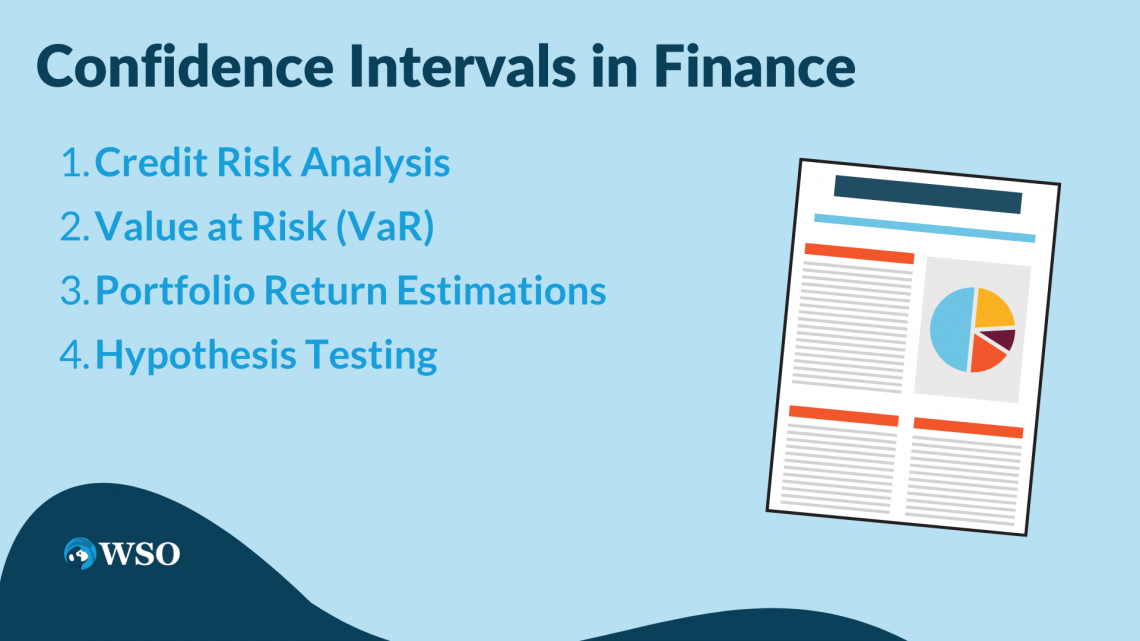
A few occasions where confidence intervals are applied in finance include:

1. Credit Risk Analysis

Confidence intervals can be set to determine a borrower's default probability at a specific confidence level. This would allow a credit risk analyst to make more informed lending decisions.

Similarly, they estimate the range of losses once a borrower has defaulted. A credit risk company needs to quantify the maximum loss with a certain degree of confidence to prepare for future defaults by borrowers.

2. Value at Risk (VaR)

The VaR calculation tells financial institutions the level of cash that must be set aside to cover a portfolio's maximum potential loss on any given day. 

3. Portfolio Return Estimations

It is difficult to use historical returns to estimate expected returns for the upcoming year. This is because past data is an unreliable metric for predicting future returns.

Hence confidence intervals are a better measure as they provide portfolio managers with a range of possible returns based on the confidence level they seek.

4. Hypothesis Testing

One can use confidence intervals in finance to test hypotheses regarding the correlation between the mean returns of Stock A and the average return of the market benchmark.

This is achieved by creating a null hypothesis (Stock A and market returns are correlated) and an alternate hypothesis (Stock A mean returns do not correlate with average market returns).

Once the two hypotheses are set, comparing the calculated confidence intervals for mean returns to the null hypothesis will provide evidence on whether the hypothesis that Stock A and market returns are correlated should be accepted or rejected.

These are some of the many applications of confidence intervals in finance. An example exploring the Value at Risk calculation further illustrates its importance. 

Confidence Intervals Example (Value at Risk) 

Value at Risk, or VaR, is a crucial risk management tool that utilizes the concept of confidence intervals to estimate the maximum loss a portfolio could experience within a certain time frame at a chosen confidence level.

Its uses extend to regulatory compliance, where corporations manage their VaR numbers to meet regulations and protect investors. Similarly, portfolio performance can be evaluated based on the ability to minimize VaR at different confidence levels.

Example 1: The first example looks at a $15 million bond portfolio; its standard deviation is 2.65%, and the desired confidence level is 95%. What is the VaR for this portfolio over a one-month horizon?

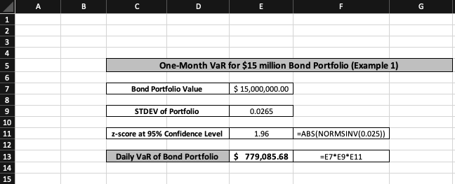
It is difficult to directly calculate the VaR over one month. Hence, the easier solution is to first compute the daily VaR for the portfolio. The daily value at risk has three components in its calculation.

Daily VaR = Portfolio Value * z-score at 95% Confidence Level * STDEV of Portfolio

The z-score at 95% confidence level was previously found to be +1.96. The logic behind it was taking the absolute value of “=NORM.S.INV(0.025)” since it is a two-tailed test wherein 2.5% on either side would equate to the remaining 5%.

The daily VaR for the bond portfolio was found to be roughly $779,086. It can be stated with 95% confidence that the maximum loss potentially incurred by the $15 million bond portfolio is $779,086 on any given day.

After finding the daily VaR, it becomes much easier to compute the one-month VaR. First, the month must be represented as 30 days; now one simply multiplies the daily value at risk of the bond portfolio by the square root of 30.

One-Month VaR = Daily VaR * √30

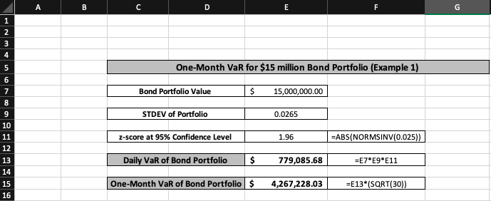
The one-month VaR for the $15 million bond portfolio is calculated as around $4,267,228. This means one can state with 95% confidence that a $15 million bond portfolio would face a maximum potential loss of roughly $4.267 million over the course of one month.

While the previous example dealt with a portfolio consisting solely of bonds, it is crucial to know the risks involved when a portfolio comprises multiple stocks.

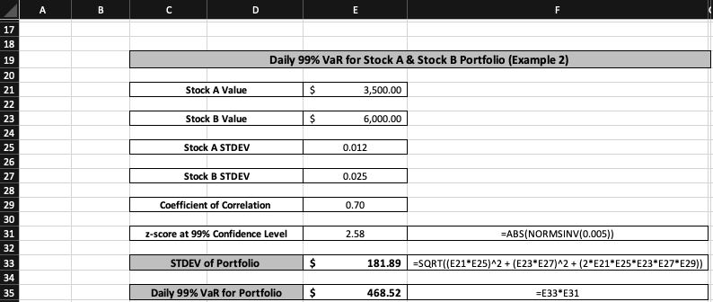
Example 2: A portfolio where $3,500 is invested in Stock A, and $6,000 is invested in Stock B. Stock A's standard deviation or volatility is 1.2%, while the volatility levels of Stock B are at 2.5%.

It is essential to mention that the coefficient of correlation between Stock A and B is 0.7. Using the information above, what is the daily VaR for this portfolio at a confidence level of 99%?

This cannot be calculated directly. First, the standard deviation of the entire portfolio must be found, and then one can move on to the daily VaR calculations. The standard deviation of the portfolio can be expressed as:

STDEV Portfolio (where A = Stock A and B = Stock B)

After finding the standard deviation of the portfolio, the daily VaR calculation at 99% confidence level is straightforward.

Daily 99% VaR = STDEV Portfolio z-score at 99% confidence level

The portfolio’s standard deviation is represented as $181.89, which implies that the portfolio value is moving away from its mean on either side by roughly $182.

When finding out the z-score at a 99% confidence level, the same two-tailed logic is used wherein the absolute value of “=NORM.S.INV(0.005)” is taken, which gives a z-score of 2.58.

The daily 99% VaR for a portfolio consisting of stocks A and B can be calculated to be $468.52. This means that it can be said with 99% confidence that a portfolio with stocks A and B would have a maximum potential loss of $468.52 on any given day. 

Importance of Confidence Intervals 

Confidence intervals are essential in letting researchers and analysts make more accurate decisions by quantifying the range of possible values for a population parameter.

Confidence levels add legitimacy and provide a concrete measure of uncertainty for the intervals. 90, 95, and 99% are common levels of confidence and strengthen the conclusions drawn using intervals.

Without its existence, there would be far less precision in estimates, which can subsequently lead to false conclusions. This would be particularly dangerous in clinical trials where treatments can be passed off as effective without the due diligence provided by intervals.

There is constant uncertainty surrounding financial data. To navigate through this, reliable estimates for price ranges are needed. An analyst cannot make informed decisions if statistical accuracy is missing from the data sample.

Additionally, the standardized nature of confidence intervals allows for comparisons between the accuracy of different studies. It can be used across various industries, making it an incredibly versatile calculation.

It also helps in identifying potential sources of error and reduces bias. The estimate has a large degree of uncertainty if the intervals calculated are wide.

By further examining the confidence intervals alongside the confidence levels, researchers can locate potential sources of error which might have contributed to increased uncertainty.

Overall, confidence intervals are a critical tool that increases the reliability of statistical inferences, which is crucial in many fields, including medicine, statistics, and finance.

Researched and Authored by Amrit Kachroo | LinkedIn 

Reviewed and Edited by Wissam El Maouch | LinkedIn

Free Resources

To continue learning and advancing your career, check out these additional helpful WSO resources:

• CRITBINOM Function
• CUMIPMT Function
• DATE Function
• DAY Function
• EFFECT Function