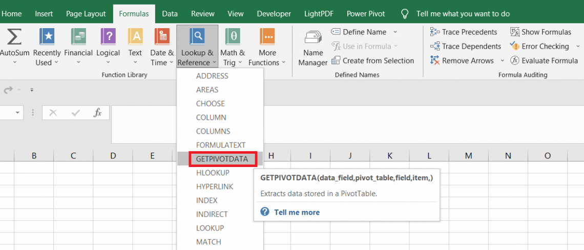
GETPIVOTDATA Function

GETPIVOTDATA function in Excel helps in data extraction from specific fields of a pivot table.

Pivot tables are one of the most essential tools for data analysis and reporting present in Excel. It allows the user to analyze large and complex data by breaking it into simpler summarized datasets.

The data can be aggregated into categories such as dates, regions, or even products, making the comparison between different line items a lot easier.

 Not only is the data perfectly summarized with precision to avoid errors, but it is also customizable by filtering, sorting, and rearranging the data in ascending or descending order.

All these pros have made pivot tables an indispensable tool for Excel users, just like how Saul Goodman was for Walter White.

When the pivot tables are extremely large, it is only natural that a function should allow you to extract the data from a specific cell. That functionality is fulfilled by the GETPIVOTDATA function.

This article will show the GETPIVOTDATA function, how to use it, and a couple of examples.

What is the GETPIVOTDATA function?

GETPIVOTDATA is categorized as a lookup and reference function that helps extract data from the specified fields of the pivot table.

For example, assume you have sales for four different regions North, South, East & West.

We want to calculate the total sales in all four regions from the Pivot Table. This can be easily done with the help of the GETPIVOTDATA function, which will extract the data from the pivot tables.

The syntax for the function is:

=GETPIVOTDATA( data_field, pivot_table, [field1, item1],[field2, item2]...)

where,

• data_field: (required) the field name that we are looking for
• pivot_table: (required) reference to the cell or range of cells 
• field1/item1: (optional) field/item pair number 1
• field2/item2: (optional) field/item number 2

Example for the GETPIVOTDATA function

Finally, let’s head over to the example of how the function works. This section will also help you refresh your memory of how to create pivot tables in Excel.

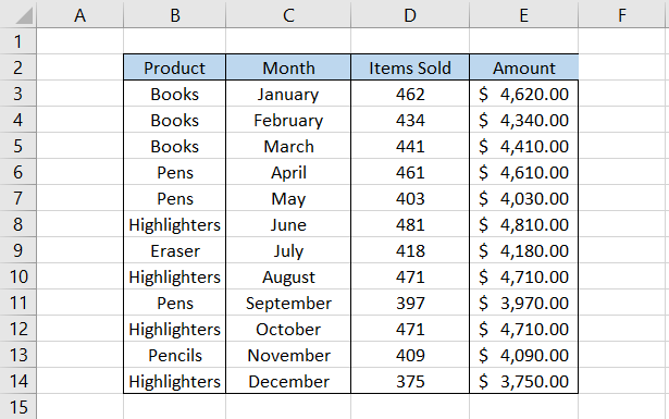
Suppose we have the data for highest selling product for each month as illustrated below:

Creating the Pivot Table

To create a pivot table, select the entire table from cell B2 to cell E14 and then click on Insert > Pivot table, which opens the below window:

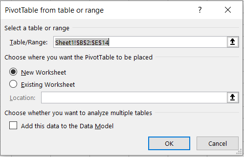
We always prefer to create the pivot table on a ‘New Worksheet,’ but you can also opt for the Existing Worksheet. The only drawback is that if the worksheet is crowded, you might find it difficult to work on the pivot table. So, finally, click on Ok.

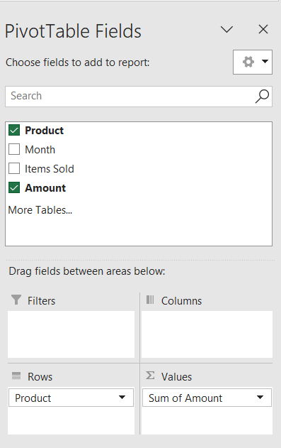
You will see a header called Pivot Table Fields on the right-hand side. This will allow you to drag different fields from the table and create the pivot table per your requirement.

For example, we dragged the ‘product’ field into the rows while the ‘amount’ field was dragged into the values area.

This gives the total sales amount for each product from the table as illustrated below:

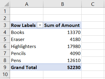
As you can see, no formulas have been used so far, and we were accurately able to return the sum total of sales for each of those unique line items present in the table.

According to the pivot table, the highlighters accounted for the highest, $17,980, whereas the pencils accounted for the lowest, $4,090.

Using the GETPIVOTTABLE function

Now that the pivot table is created, let's try and use the GETPIVOTTABLE function.

Suppose we want the total sum of all the items from the given pivot table. We will use the formula =GETPIVOTDATA("Sum of Amount",B3), which gives the result as:

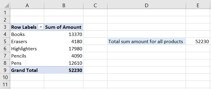
Thus, by referencing the field name and cell address, we got the sum total of all the products in our dataset.

What if we wanted to get the sum total of individual products? How would the formula change to get those values?

Suppose we want the total amount for the highlighters sold in our given dataset. Then, we will use the formula =GETPIVOTDATA("Amount",$A$3,"Product","Highlighters"), which gives the result as:

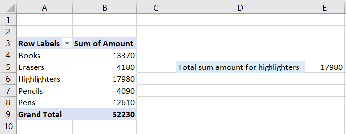
What we did was first capture the field name from the table, i.e., ‘Amount,’ and then referenced the corresponding cell in the pivot table and then referenced another field name from table ‘Product’ to finally input the final text string as ‘Highlighters’ to get the sum total amount.

But we hear you. This formula can be quite tricky to write, and you might need to revisit the table now and then to see what the table field names are.

Do you know what's simpler than that?

Begin the formula with an equal sign (=), then reference the cell whose value you want to extract from the pivot table. That’s it.

You will see that the formula in the cell will be

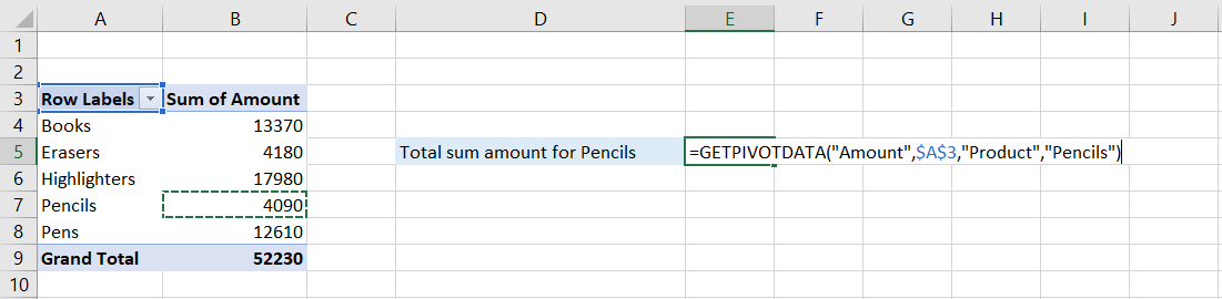
This way, you can eliminate all the hassle of individually writing the formula and making things more complicated for yourself.

I know I should have said this earlier, but it is equally important to understand the construct of a function before using it.

Practical Example of Getpivotdata Function 

Let’s make our pivot table a bit more complicated. Suppose you are a day trader and take intraday positions in two stocks: Microsoft Inc and Meta Platforms Inc.

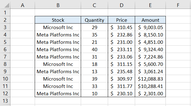
To create the pivot table from the data, we will select the range from cell B2 to cell E12 and then click on Insert > Pivot Table.

We will create the pivot table on a new spreadsheet wherein we will next drag the fields into the respective areas on the pivot table fields pane.

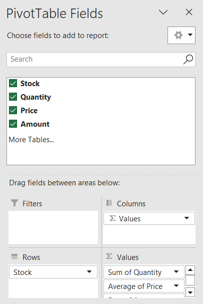
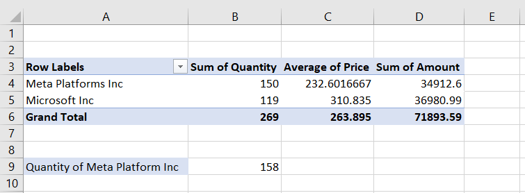
Here, we have added the ‘Stock’ field to the row areas while the rest of the fields are added to the Values area. Amongst those three, the two, i.e., the Quantity and Amount, will be represented as the sum total, whereas the price will be represented as the average value.

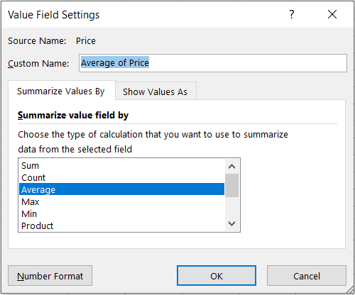
To change the type of calculation for a dragged field, you only need to right-click on it and then select the Value Field Settings option. This will open up a dialog box wherein you need to click on ‘Average’ to eventually display the stock's average price.

Finally, we come to the best part of the article, which is using the GETPIVOTDATA function. Again, we will use the easier method but with some variations.

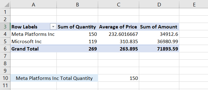
First, let’s extract the total quantity of Meta Platform Inc from the pivot table. We will begin with the equal sign, directly reference cell B4, and press Enter.

If we press the F2 key in the cell, it will display the formula as =GETPIVOTDATA("Sum of Quantity",$A$3,"Stock","Meta Platforms Inc") to give the result 150.

Suppose you want to know the difference between the total amount spent on trading Meta Platforms Inc and Microsoft Inc.

Here, we will just reference both cells and subtract them from each other. The formula becomes =D5-D4 to give the result of $2,068.39.

However, if you press the F2 key, you will find that the formula is =GETPIVOTDATA("Sum of Amount",$A$3,"Stock","Microsoft Inc")-GETPIVOTDATA("Sum of Amount",$A$3,"Stock","Meta Platforms Inc"). So it is the same thing, but yea a bit complicated!

Suppose you want to know how many Meta Inc stocks you can buy in the total amount you bought Microsoft Inc, which is $36,980.99.

We also have the average price of Meta Platforms Inc, which is $232.60. Thus, all you need to do is use the formula =D5/C4 -1, which gives the result of 158.

The formula then actually becomes =GETPIVOTDATA("Sum of Amount",$A$3,"Stock","Microsoft Inc")/GETPIVOTDATA("Average of Price",$A$3,"Stock","Meta Platforms Inc")-1 to give the result:

You must be thinking, why subtract one from the result? Well, it’s just a preference. We have assumed the stock's average price, which will likely change when you make an original order for stock.

Thus, buying one quantity less gives you that cushion so the purchase order does not exceed the investment value.

Researched and authored by Akash Bagul | LinkedIn

Reviewed and edited by Parul Gupta | LinkedIn

Free Resources

To continue learning and advancing your career, check out these additional helpful WSO resources:

• BINOM.DIST.RANGE Function
• CEILING.PRECISE Function
• DATE Function
• DAY Function
• DISC Function