MODE.MULT Function

What is the MODE.MULT Function?

The MODE.MULT function returns a vertical array of recurring values, i.e., the ones making the most appearances in our dataset.

Hmm, something sounds familiar.

Wait, isn't that something we used to do in school? We used to calculate the MODE in math class, where the number making the most appearances would be our result from the given dataset.

But how does the function differ from the traditional mode?

The most significant difference that you would find between both is that MODE.MULT helps to return all the values that make the most appearances in a given dataset. If three values make equal 'n' appearances, then the function returns all three as an array.

As a financial analyst, the function helps to highlight the most frequently occurring numbers or dates from the given dataset.

How The MODE.MULT function work?

The MODE.MULT is categorized as a Statistical function that returns the array of values with the maximum number of occurrences within a given dataset.

Traditionally, when you use the MODE function in Excel(yes, a MODE function exists as well, which we will cover in subsequent sections), it returns just a single value that made the maximum appearances in the dataset.

For example, if you have the number 12,12,13,13,13,15,11, then the MODE function will return the result as 13.

If there are two numbers with the same number of recurrences, for example, 12,12,13,13,14,15, then the function will return the result as 12 since it is the first number with the maximum appearance in our dataset.

Do Y'all think this is fair for number 13?

Nope. This is where the MODE.MULT function would return both the numbers as a result of an array, i.e., 12 and 13. If the numbers were 12,12,13,13,14,14,15, then the function would return the result as 12,13, and 14.

The syntax for the function is:

=MODE.MULT(number1,[number2]...)

where,

number1 - (required) the first number or the range of numbers

number2 - (optional) the second number or the range of numbers

How to use the MODE.MULT function?

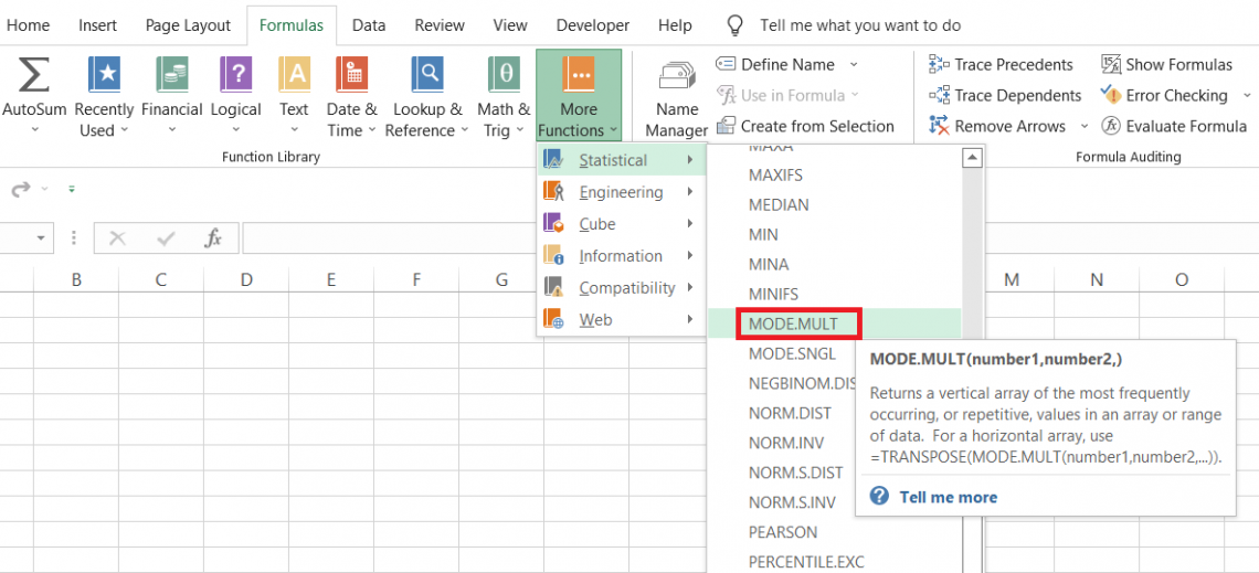
The function does not have complicated arguments to begin with. You can reference the range of cells or cells in the process or directly hardcode the values. One of the two methods to use the function is to select it from the function's library.

Click on the Formulas tab > More Functions > Statistical > and select the MODE.MULT function from the drop-down menu.

This will open up the dialog box where you input the arguments or reference the numerical values.

For example, we have input the numbers 2, 2, 3, 2, 3, 2, 3, 3, and 1 as our argument in the dialog box.

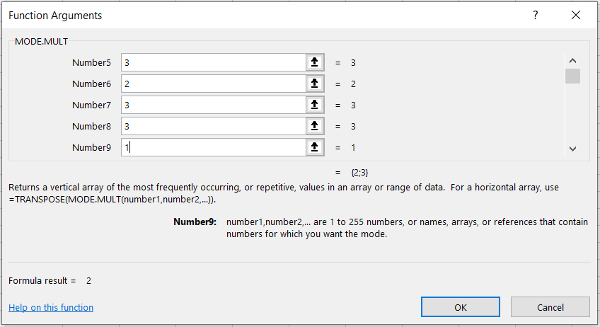
The maximum number of occurrences is for numbers 2 and 3, which appear four times, respectively.

Thus, we get the array of those numbers; as a result, i.e., {2,3} as represented below the arguments in the dialog box. Once you click on Ok, you should get the same effect in the selected cell.

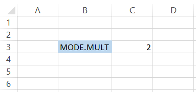
Wait, what? Why did we get only one number as our result?

There was one mistake that we made before using the function. Since this is an array-based formula, we need to select a range of cells in which we expect the multiple mode values.

Should we go through the function's library again to use the function? You can also use the function as the worksheet formula, a quick method that saves time.

First, we select the range of cells as illustrated below:

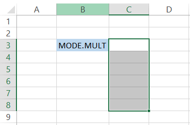
Next, we type the formula in cell C3 with cells still highlighted. Again, it doesn't matter how many cells you select. Just ensure that there are ample cells to accommodate multiple mode values.

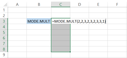
Finally, press the Ctrl + Shift + Enter keys on the keyboard to run the array formula, which gives you the result:

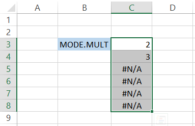
As you see, we get both the mode values as our result. Since there are no recurring maximum values in our dataset, the rest of the selected cells return the #N/A error.

As we said, it doesn't matter how many cells you select, the function returns the result in the required cells, and the rest(even if you cannot delete) return the #N/A error.

Note: An important thing to remember is to select the range before using the formula only in Excel versions apart from Excel 365. 

The latter version dynamically spills the array values into multiple cells, i.e., you don't even need to press the Ctrl + Shift + Enter key on the keyboard to use the formula.

Example for the MODE.MULT function

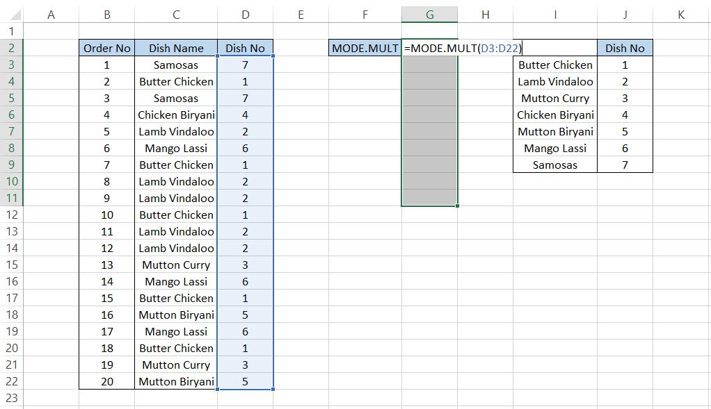
Let's say you run a restaurant specializing in Indian cuisine and need to find some of the best-selling items on your menu. So you decide to evaluate all the sales for a single day and see the gems on your menu.

All the sales(individual items) made from your restaurant are as illustrated below:

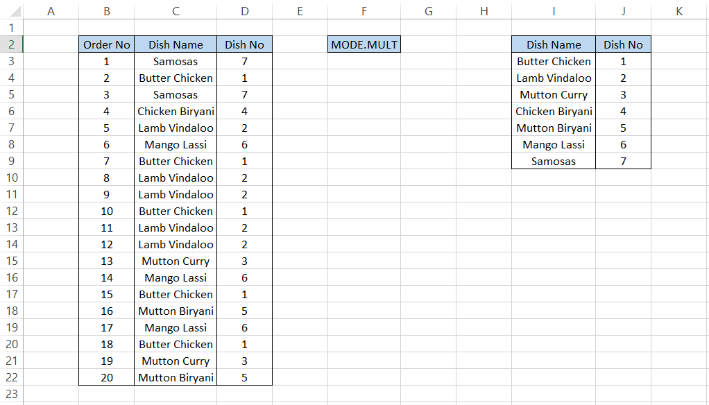
Since the MODE.MULT function cannot identify text strings; we have assigned unique numbers to those text strings as in column J.

The formula that we will use in cell G4 will be

=MODE.MULT(D3:D22)

will give us the maximum number of dishes sold as 1 and 2.

If you check those two dishes in columns I and J, you will find Butter Chicken and Lamb Vindaloo.

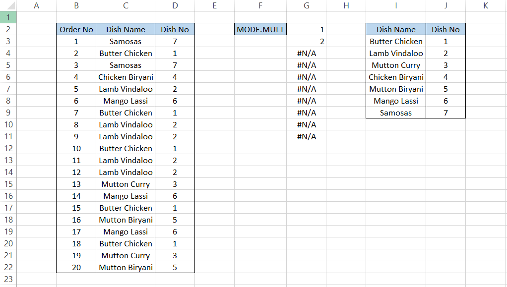
Thus, using the MODE.MULT you can easily find, in this case, the best-selling dishes in your restaurant. Also, just some advice from us - you all might need to work on that Chicken Biryani. 

As the OG Mukbanger Quang Tran once quoted in his YouTube video (timestamp-11:58 -12:22), you can tell a restaurant's ratings by their Biryani…their Chicken Biryani. So if the Biryani is good, you know the rest of the menu is good too".

If you wish to return the vertical array as a horizontal array of values, you can nest the formula inside the TRANSPOSE function.

However, you will need to select the horizontal range of cells first and then use the formula as illustrated below:

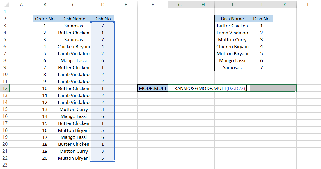
The formula will be

=TRANSPOSE(MODE.MULT(D3:D22))

which gives you the maximum occurring values as 1 and 2.

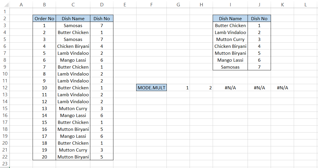
Thus, the MODE.MULT is an array-based formula that will return multiple mode values based on their occurrences in the dataset.

what is the MODE Function?

The MODE is a Statistical function; however, you will find it under the Compatibility section. As you might have already guessed, the function returns a single value with the maximum number of appearances in the given dataset.

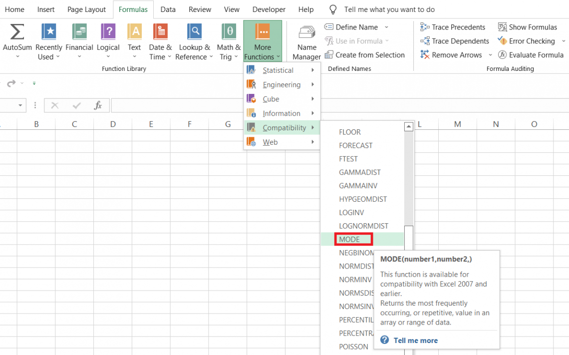
The MODE was the preferred version for getting the value of maximum occurrences before it was replaced by two newer versions, one of which is the MODE.MULT.

However, you can still use the backward compatibility function in the latest Excel versions.

There isn't much difference in the syntax for the function, i.e., the same arguments exist. The only thing that changes is the function name and the result it returns.

The reason that Excel had to replace the function with newer alternatives is to offer the users more flexibility in terms of returning the desired result. Therefore, we can say that the objective was established by introducing the MODE.MULT function.

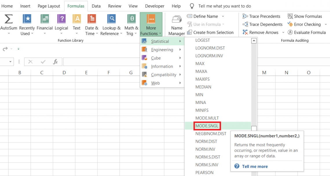
What is the MODE.SNGL function?

The other newer version, which was introduced in place of the MODE function, is the MODE.SNGL. This function is closest to what Excel previously offered in the MODE function.

The MODE.SNGL function returns the single value that makes the most number of appearances in the given dataset.

You would probably think - "Why were two functions introduced rather than just MODE?MULT?"

It could be something to do with maintaining consistency in naming the function, or maybe they have plans to introduce another similar function. 

The dot(.) helps branch the main function into various subsets offering Excel users greater flexibility while working on spreadsheets.

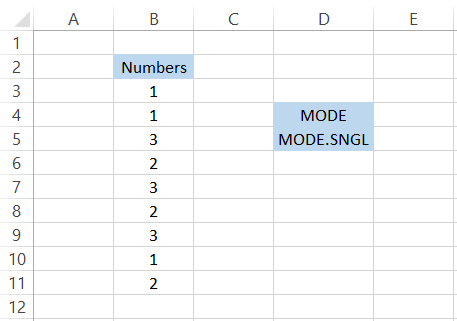
Since we skipped the example in the previous section, we will make a comparative analysis of MODE and MODE.SNGL to understand whether they return contrasting results. 

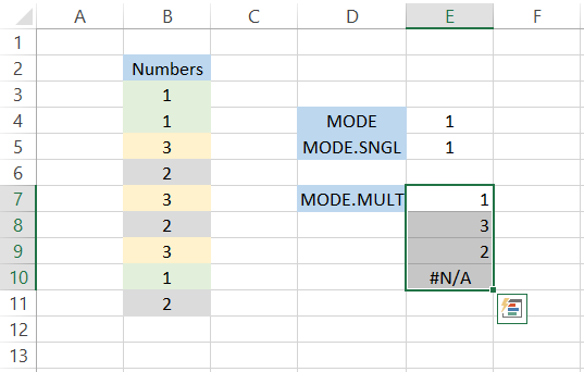
Suppose that some numbers in Excel as illustrated below:

By using the formula

=MODE(B3:B11) in cell E4 and =MODE.SNGL(B3:B11)

in cell E5, we get the result of 1 in each cell.

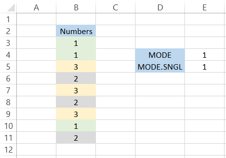
Even though we have each number an equal number of times, we still get the result as one since both the functions identify the number as the first number with the most recurrences in the given dataset.

Thus, you can use either of those two functions if you need to find only a single value that makes maximum occurrences in a given dataset.

Otherwise, select the range of cells, and type in the formula

=MODE.MULT(B3:B11)

which gives the result:

Text Strings and MODE function

We all agree that each MODE function doesn't collaborate directly with the text strings. Text strings aren't numbers that can be compared; we would accept that you could compare boolean values traditionally using the MODE function but text strings?

Absolutely not.

However, is it true?

There are some loopholes, or the usage of multiple functions allows you to find the most frequently occurring text strings using the combination of INDEX, MATCH, and MODE.MULT function.

Let's say you have the trading data as illustrated below:

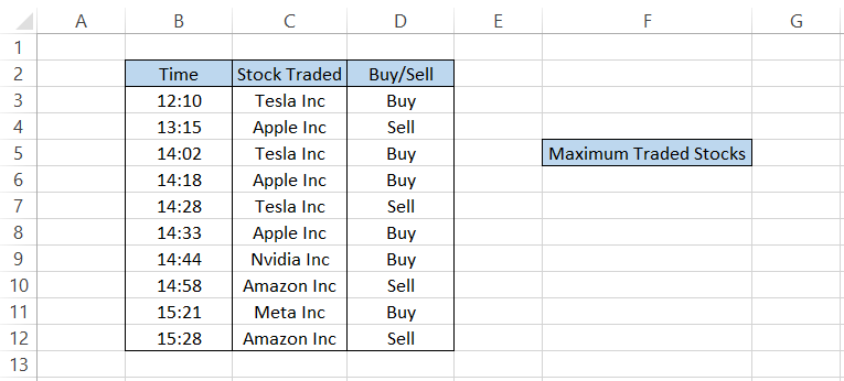
To find what the most traded stocks are, we will first select the range of cells and then use the formula

=INDEX(C3:C12, MODE.MULT(MATCH(C3:C12, C3:C12,0)))

In cell G5, which gives the result:

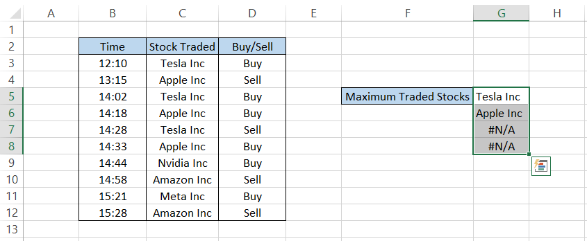
The two most traded stocks are Tesla Inc and Apple Inc, respectively. Therefore, if we wanted to find a single value making maximum appearances in the dataset, we would have replaced the MODE.MULT with either of the other two functions.

Since this is also an array formula, you must press Ctrl + Shift + Enter to get the result.

How does the formula work?

• Firstly, the MATCH function in combination with the MODE.MULT identifies the position of the text strings that makes maximum appearances in the given dataset.
• Once those text strings are identified, the INDEX function extracts those same values, and we get the result in the selected cells.
• If we select additional cells, we get the result as #N/A, indicating no mode values in the dataset.

Conclusion

Excel's MODE.MULT function is a major step forward in data analysis capabilities, especially in cases when datasets have many recurring values and complex distributions.

Compared to the MODE function, MODE.MULT provides a more thorough comprehension of data patterns because it returns an array of numbers that represents every mode in the dataset.

Thanks to this increased functionality, users in various industries, including finance and inventory management, may now extract deeper insights and make better decisions.

MODE.MULT proves to be a potent tool for extracting deeper insights from datasets, allowing users to improve workflows, spot trends, and achieve better results.

Free Resources

To continue learning and advancing your career, check out these additional helpful WSO resources:

• HOUR Function
• HYPERLINK Function
• PEARSON Function
• PI Function
• SEARCH Function