UPPER Function

What Is The UPPER function?

The UPPER function in Excel converts all the letters in a text string to an uppercase version.

Imagine the number of times you were in a hurry to leave for home, and all that was left was to send out an email to the client. So you hurriedly type in the email, not even looking for a second at the screen.

Midway through, you glance at the screen, and to your horror, you have been typing the entire email in capitalized text strings!

The Caps Lock key was left on, you did not notice, and now you need to fix it all over again before you can finally send the email.

Typing the email in uppercase was a mistake, but an Excel function will intentionally let you return a text string in the uppercase version.

You’ve guessed it right. Dumbledore would be proud; 10+ points to Gryffindor! The function is none other than UPPER.

In this article, we will see the syntax for the function and a couple of examples of how to use the function.

Understanding The UPPER function

The UPPER is categorized as a text function that converts the supplied text strings into a capitalized or uppercase version.

Irrespective of what text you type in Excel, the function will identify all the characters/letters in lowercase and return them in uppercase. The characters which are already in uppercase will be left unchanged.

For example, if you have the text string as ‘Ethereum’ and use the function on the text string, you will get the result as ‘ETHEREUM.’

Even if the text string has a delimiter character, such as a space separating multiple substrings, still the function will return the entire text string in capitalized format.

For example, if you have the text string ‘711 is the average credit score in the United States' and use the UPPER function, you will get the result ‘711 IS THE AVERAGE CREDIT SCORE IN THE UNITED STATES.’

We noticed that even though we had numerical values in our text string, the function did not affect it. Hence, a conclusion can be made that the function does not affect numerical values, punctuations, or even space characters.

UPPER Function Formula

The syntax for the function is:

=UPPER(text)

where,

text - (required) the reference to the text string, which will be returned in the uppercase version.

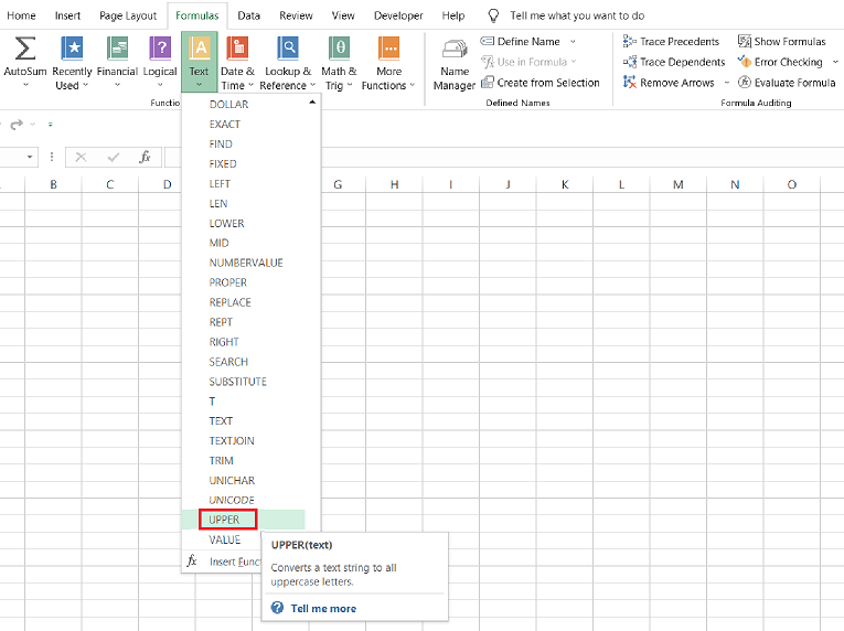
How to use the UPPER Function in Excel?

A single argument function becomes easy to use where the argument can either be hardcoded or input as a single cell reference.

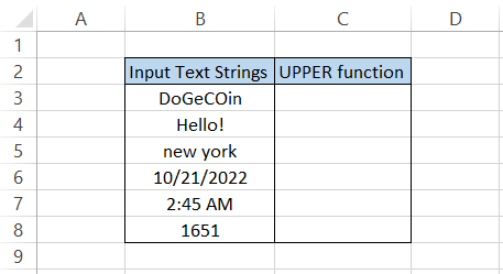
Suppose you have the data in Excel as illustrated below:

Then, to use the function as a worksheet formula, we begin with an equal sign, type in the function name, and reference the cells in column B inside the parentheses.

The formula in cell C3 will be =UPPER(B3), which you can drag to cell C8 to give the result:

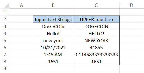
As we had previously mentioned, all the characters in lowercase are capitalized, while the characters already in uppercase remain unchanged.

We had the exclamation punctuation in cell B4. However, the function did not affect it, and the punctuation returned along with the result.

Cell B8 has a numerical value equal to 1651. Since the ‘text’ function finally focuses on text strings, the numerical value is unaffected by the effect of the function.

The only noticeable effect of the function is that it removes the format for date and time values.

The date is returned as its serial number equivalent, while the time loses its format to return as a decimal number.

UPPER Function Examples

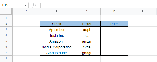
Suppose you download the stock price quotes from a third-party website. You are looking to 

import real-time stock data directly into Google Sheets.

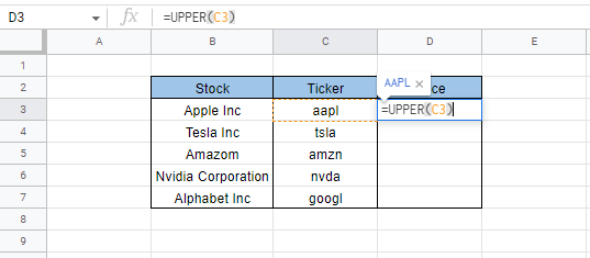
The issue, however, is that the ticker symbol for the stocks is imported all wrong(lowercase), as illustrated below:

To change the ticker symbol directly rather than manually changing them, we will use the formula =UPPER(C3) in cell D3 as below:

We will get the result as AAPL in cell D3. Then, finally, dragging down the formula to cell D7, we get:

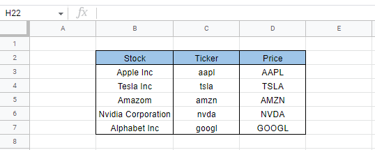
However, our data does not match our column headers. So, we will PasteSpecial the values in range D3:D7 and copy them in range C3:C7.

Now, all you need to do is use the =GOOGLEFINANCE(C3) in cell D3 and drag it down to cell D7, which gives us the stock prices as

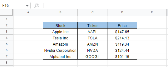
The amazing thing about the GOOGLEFINANCE function is that it will automatically update the stock price after a delay of up to 20 minutes.

There are a lot more different attributes that you can pull through the GOOGLEFINANCE function, but we will probably save it for some other day.

For now, remember that the UPPER function will return the text string in the uppercase version.

Returning to Excel, there’s a scenario where you can use the UPPER function and the Data Validation tool to accept values only in uppercase.

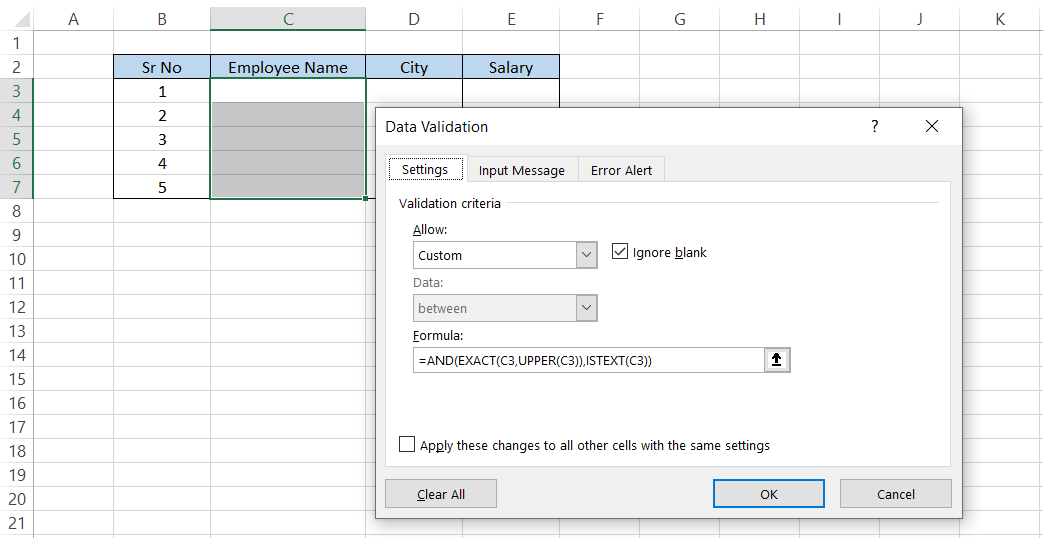
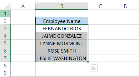
For example, suppose you have an Employee database where the Employee name must always be in capitalized format.

To ensure that only the text strings in uppercase are accepted as the value, we will select the range C3:C7 and click on Data > Data Validation Tool.

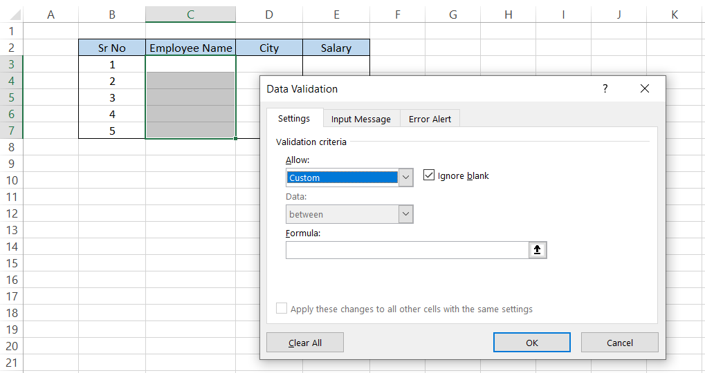
Here, we will select the ‘Custom’ Value and type in the formula as =AND(EXACT(C3,UPPER(C3)),ISTEXT(C3)), and click on Ok.

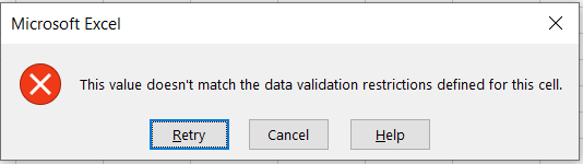
Suppose you type in text in column C now. In that case, you will find that the cell accepts text strings only in upper case, or else it will return the error as

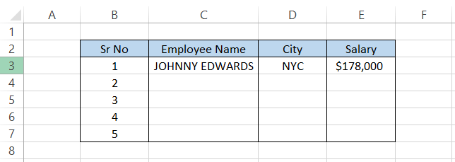
You can use the formula and the data validation tool for multiple columns in which you intend to input the values in capitalized format.

Only when you input the text string in the capitalized format, the cell accepts those values and store them in the cell as:

UPPER vs. LOWER function

A function that works exactly opposite to the UPPER is the LOWER function.

The LOWER is categorized as a text function that returns the supplied text string in a lowercase version.

For example, if you have the text string as ‘HeLLo’ and use the LOWER function, you will get the result as ‘hello.’

The characters which are already in lowercase remain unaffected, while the character/letters which are in uppercase or capitalized change into lowercase.

Another thing we need to remember is that the function will completely ignore numerical values, punctuations, and space characters in the result.

Example

Let’s see an example of how the results for both functions compare.

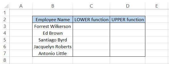
Suppose you have the data in Excel, as illustrated below:

By using the formula =LOWER(B3) in cell C3 and dragging it down to cell C7, we get the result as

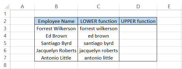
As you can see, irrespective of whether the characters are in upper or lowercase, the result is ultimately in lowercase.

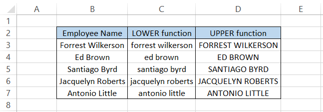
Similarly, we will use the =UPPER(B3) in cell D3 and drag it down to cell D7, which gives the result:

UPPER vs. PROPER function

A text manipulation function that all Excel users should know is the PROPER function.

The PROPER is categorized as a Text function that accepts a supplied text string and returns the first letter of a text string in uppercase, while the rest is returned in a lowercase version.

As the name and the category for the function suggest, its role is to return the text string in the ‘proper’ format.

A lot of times, data imported from third-party websites might not be in a readable or acceptable format.

At such times, rather than retyping the changes in Excel, you need to use the PROPER function to fix the text issue in seconds.

For example, a text string such as ‘APplE inC’ will return as ‘Apple Inc’ when you use the PROPER function.

An important thing to remember is that if a space character separates a substring, then the next substring's first letter is again capitalized.

For example, in the case of ‘Apple Inc,’ the substring ‘Inc’ was separated by a space character and returned as capitalized.

The same will apply if numerical values or punctuation marks exist in a given text string.

The syntax for the function is:

=PROPER(text)

where,

text = (required) a text string enclosed inside the quotation marks, a cell reference for the text strings, or a formula that returns a text value.

Example

Let's see a simple example of how the results would compare for both functions.

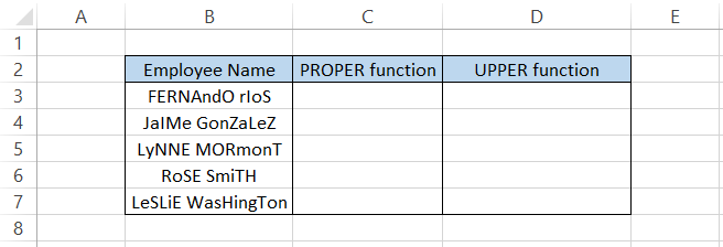
Suppose that you have the data in Excel as illustrated below:

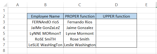
To return the employee names in the ‘proper’ case, we will use the formula =PROPER(B3) in cell C3 and drag it down to cell C7, which gives the result:

Similarly, we will use the formula =UPPER(B3) in cell D3 and drag it to cell D7. We get:

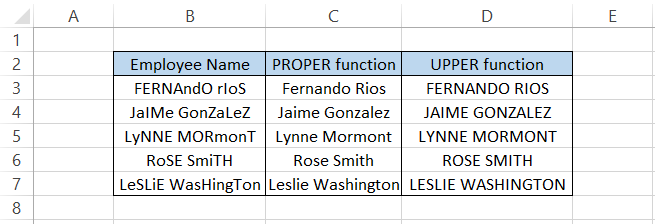
The difference in the result that both the function’s yield is quite evident. However, as we always say - “Each function has its capabilities that can be used to advantage in certain scenarios.”

It is entirely up to you how you leverage the power of different functions to the full of their capabilities.

VBA code: Return text string in uppercase

If you have been correcting text strings to uppercase daily, wouldn’t it make sense to automate this repetitive task?

Yes, you are right. You can write a VBA code that will return the text string in uppercase for the selected range of cells.

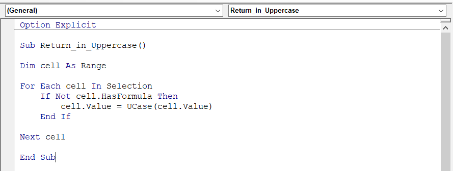
The snippet of code that will be used is illustrated below:

Now, if you select a range of cells consisting of text strings and run the VBA code, you will get the result as

No hassle creating additional columns or PasteSpecial values in another range of cells.

However, it's not feasible to always go into the developer tab and run the macro after selecting the range of cells.

In this case, you can opt for two options:

• Creating a VBA button and assigning the VBA code to it so that it will run the code with just a single click.
• Add the macro in the ribbon so the VBA button does not take up additional space in the spreadsheet.

Since we all know how to add a VBA button, perhaps it makes sense to explore ‘adding a macro to the ribbon option.’

The steps you need to follow are:

• Click on File > Options > Quick Access Toolbar
• Select ‘Macro’ under the Choose commands from the drop-down menu.
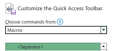
• You will see all the different VBA codes that you have written. Next, select the one you intend to add to the ribbon, which is Return_in_Uppercase.
• Click on Add and select the macro. You can also edit the icon for the macro based on what the code does by clicking on ‘Modify.’ For example, we changed the icon to
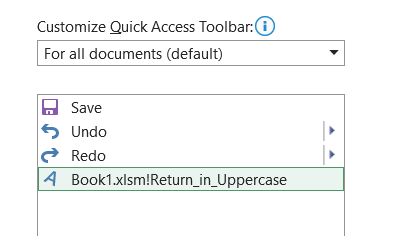
• Finally, click on Ok, and you will find the icon for the macro in the ribbon.

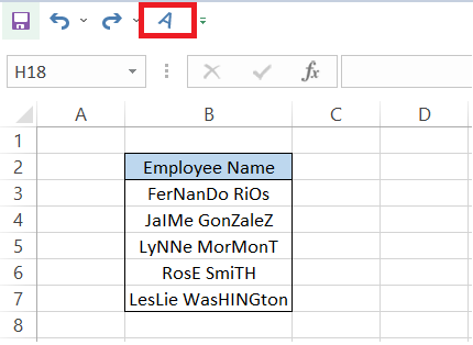
Now, select the range B3:B7 and click on the icon to run the macro, and it will do the rest of the work.

Researched and Authored by Akash Bagul | Linkedin

Reviewed and edited by Parul Gupta | LinkedIn

Free Resources

To continue learning and advancing your career, check out these additional helpful WSO resources:

• TRUE Function
• VAR.P Function
• WORKDAY Function
• XIRR Function
• XOR Function