ROUNDUP Excel

What Is Excel ROUNDUP?

The ROUNDUP function in Excel rounds up the number to the given decimal away from zero.

The problem with simple and complex arithmetic calculations is that sometimes you might get a result that would be difficult to interpret and rewrite in other arithmetic equations. 

For example, the value you get when you find the root of 2 equals 1.4142135623730950488016887242097. 

The use of exact results improves the precision of the calculations, but at the same time, you need to maintain this consistency throughout the entire dataset.

Since such recurring and irrational decimals make life difficult while calculating in a spreadsheet, it's best to limit them to a certain number of digits after the decimal point.

But wait! We never said what recurring and irrational decimals mean. So first, let's see what different types of decimal numbers you would encounter while working in Excel.

A decimal number can be of three types:

• They are terminating decimals - A decimal number with a finite number of digits after the decimal point. For example, when you divide 1 by 2, you will get the result of 0.5. Since the digits after the decimal point are finite, they are called terminating decimals. 
• Recurring decimals - A decimal number where the digits keep repeating in the same pattern after the decimal point. For example, 0.232323232323232, 0.481481481481481481 etc.
• Irrational decimals - Another decimal number where the digit after the decimal point keeps repeating infinitely. The digits after the decimal point are not recurring in nature. For example, 0.1423456879465132465498, 789.45613249872893964 etc

There are two main reasons why you need to round up the values.

Firstly, it makes the number easier to use. For example, hardcoding a 4.98 numerical value is much easier than 4.987984654513549879. Yes, you could reference them, but there are instances where it's just appropriate to hardcode the numbers.

You might argue that the numbers might lose a significant amount of their accuracy by rounding up numbers. But that is not the case. The number is still very close to our actual result.

For example, if you visit a Walmart and the bill comes out to $28.5648, is it possible to pay the amount up to that accuracy? Not!

In such a case, the cashier rounds up the value to two decimal places, i.e., $28.56, and returns the bill with the same amount.

In this article, we will see the syntax for the function, how to use the function, as well as a couple of examples to understand how the function works.

Understanding the ROUNDUP function

The function is categorized as a Math and Trig function that rounds a numerical value away from zero. 

The general rule when you use the function is that the 'nth' digit after the decimal point will always be greater by one than the previous value.

For example, if you have the number 28.9746 and you need to round up to two digits after decimal using the function, you would get the result as 28.98.

We always had a little exercise while studying in school about rounding up numbers where we followed a standard procedure - if the number lies between 0 to 4, we will round towards zero. In contrast, if the number at the end lies between 5 to 9, we will round away from zero.

Suppose the number is 28.984. Using our standard rules, rounding the number to two digits would give us the result of 28.98.

However, the same rule would give us the result as 29.0 if we round the value to one digit(since 8 lies between 5 to 9, one gets added to the preceding number, which again gets rounded to give the result as 29).

The function does not follow this rule and would give a rounded-up value for all the numbers due to the numerical value.

ROUNDUP Function Formula

The syntax for the function is:

=ROUNDUP(number, num_digits)

where,

• number = (required) The number which will round up to the specified number of digits after the decimal.
• num_digits = (required) the number of decimal places you want to round up the value.

How the Excel ROUNDUP Function Works

It goes without saying how easy it is to use the function. We have been studying rounding numbers our entire school life.

Even though 'Mitochondria is the powerhouse of the cell' has been the most useful in our professional lives, rounding up the numbers isn't far away.

Rounding numbers is one of the school learnings that we use in real life. So, for example, if you are a business owner, you would need this function to maintain the records, and you could do so seamlessly in Excel.

Method 1: From the functions library

If you are a beginner and just starting to work on Excel, you wouldn't know a lot of functions. So you need to explore the library first, which will help you become more confident in using the worksheet formulas.

But what exactly is a function? A function is a predefined formula wherein you input the arguments in the text boxes to get the result in the cell. To use the process, please follow the below steps:

1. Select the cell in which you want to return the result.
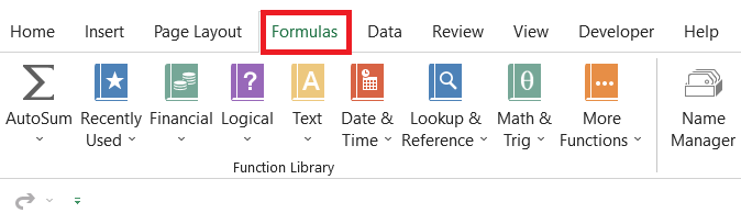
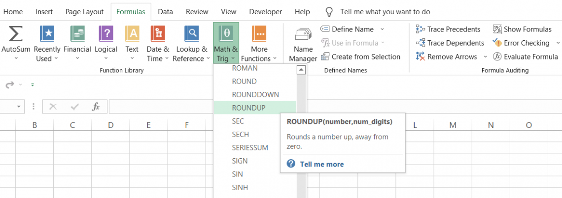
2. Next, click on the Formulas tab > Math & Trig > look for the ROUNDUP from the drop-down box.
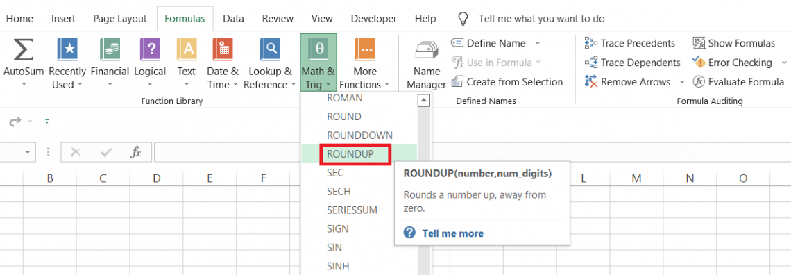
3. This will open up the dialog box as illustrated below:
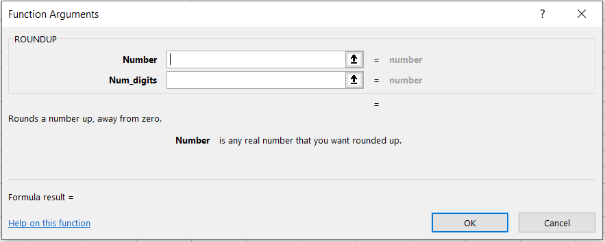
4. Next, we input the arguments in both text boxes. Either you can hardcode the values or just reference the cells directly. Here, we will input the number as 28.989 and num_digits as 2.
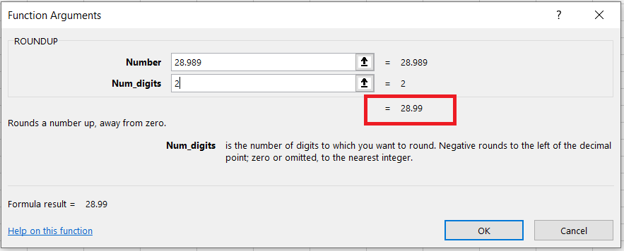
5. You might have already noticed that you get the preview of the result, as illustrated above. The result is equal to 28.99
6. Finally, all you need to do is click on Ok, and you will get the same result in the selected cell.

Method 2: As a worksheet formula

If you have a basic understanding of some of the functions in Excel, you can directly jump to using the functions as a worksheet formula.

The worksheet formula is where the real show begins. Using functions from the library has its limitations and is overcome by using it as a formula.

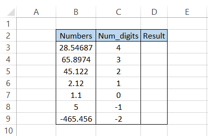
Suppose that you have numbers in Excel as illustrated below:

We will use the formula =ROUNDUP(B3,C3), which would give us the result:

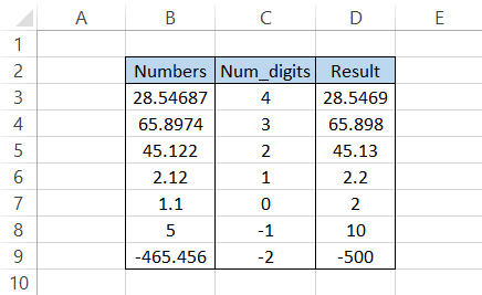
Rather than hardcoding the values, we directly reference the values in the formula, giving us the expected result.

You might have noticed that whatever digit you want to round up the number value to gets elevated in its position by one, i.e., 1 becomes 2, 2 becomes 3, and so on.

There is a rather exciting observation for 1.1 after using the formula. We round it to 0 decimal places(we mean to tell excel is remove all digits after decimal), which gives us the result away from zero as 2.

Similarly, a numerical value of 5 gives us a rounded-up value of 10. Thus, you could use zero, positive, and negative integers as a num_digits argument in the formula.

ROUNDUP Function Example

When you use the function, except the 'nth' term digit after the decimal point, to get rounded up away from zero, you would see a significant change with the function with only two arguments.

The function can be combined with math and trig functions such as SUM, AVERAGE, SQRT, etc.

Once you find the result using the math functions, if the result is a number with too many digits after the decimal point, you can nest the formula inside the function.

For example, suppose the formula =AVERAGE(A2:A15) gives the result 8.78946, then by using the updated recipe =ROUNDUP(AVERAGE(A2:A15),2). In that case, you will get the result as 8.79 by limiting the digits after the decimal to 2.

It's as simple as it sounds :)

In this section, we will see examples to better understand the function.

Example 1: Numbers

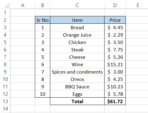
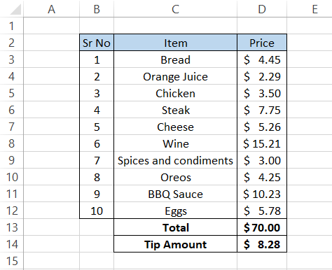
Suppose that you visit a supermarket and buy a total of ten items. The prices for the items are as illustrated below:

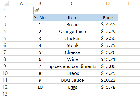
You are a generous person, so you decide to tip the cashier. Now, if you want, you can list any amount depending on what num_digit argument you use.

Firstly, we would find the total amount for all the items using the SUM function. This would give us the result equal to $61.72 using the formula =SUM(D3:D12).

Based on the understanding of the number, we can use the num_digit argument as equal to 1,0,-1,-2,-3…' n.'

To find the ideal tip amount, we will nest the SUM function result such that the formula becomes =ROUNDUP(SUM(D3:D12),1) to give the final result:

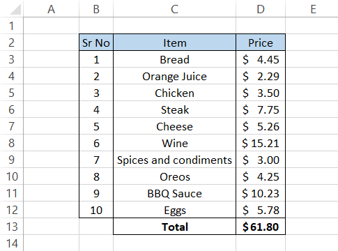
A two-cent tip? Doesn't make much sense. We will next use 0 as the num_digits argument using which formula becomes =ROUNDUP(SUM(D3:D12),0) to give the result:

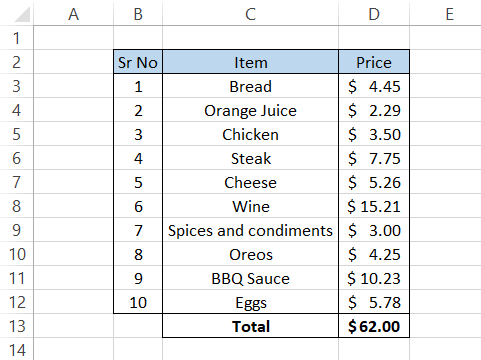
We are on the right track; finally, let's try to use -1 as our num_digits argument using the formula =ROUNDUP(SUM(D3:D12),-1)

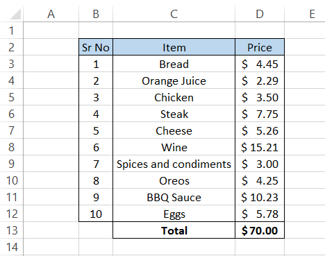
And there we have it! If you keep decreasing the num_digits argument, you will get a more significant amount which means a bigger tip.

To find the tip amount, you can use the formula =ROUNDUP(SUM(D3:D12),-1)-SUM(D3:D12), which gives the result as $8.28.

You can also directly link the formula to the total amount in cell D13 such that the procedure becomes =D13-SUM(D3:D12). This way, the tip amount automatically gets updated whenever you shift the decimal digits to round up a number.

Example 2: Date and time

The date is represented as serial numbers in Excel, while time is represented as decimal numbers.

The dates in Excel begin from 1st Jan 1900, whose serial number is equal to 1, whereas if the time is equal to 12:00 PM, then it is equal to decimal number 0.5.

You would hardly ever use the function on date and time, but you can sometimes make these mistakes unintentionally.

To see what effect the function would have on these data types, we will see an example to understand better.

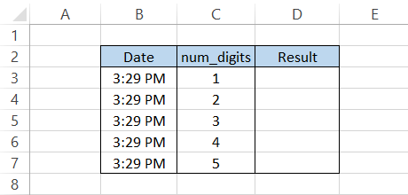
Suppose you have the data in Excel as illustrated below:

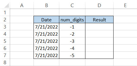
First and foremost, you can't use the positive integers or zero as num_digits arguments since it would give you the same result.

The formula that we would use to get the result in column D is =ROUNDUP(B3, C3), which gives the result:

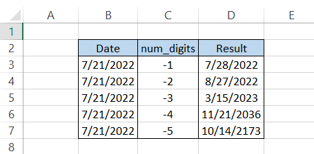
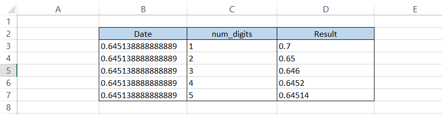
If you need to know what happened behind the scene, then press the keyboard shortcut of Ctrl + ~, which shows the serial numbers for the date as:

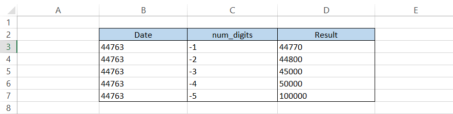
You would need to Paste the particular values before, or else you will see the formulas in column D.

Similarly, suppose that we have data for the time as illustrated below:

The scenario for time would be completely different. Since time is represented as decimal numbers between 0 and 1, using negative integers and zero as num_digits will ultimately give the result as 12:00 AM.

To find the result, we will use the formula =ROUNDUP(B3,C3), which gives us the result:

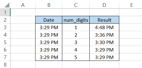
As you go away from zero for the num_digits argument, the difference in time becomes insignificant.

Again, if you need to check what happened behind the scenes, then you can use the Ctrl + ~ key after PasteSpecial the values in column D, which look as:

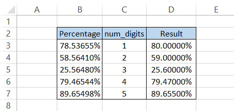
Example 3: Percentage

Here is the most critical example based on the function. Percentages are present in all databases, whether you are working on mortgage reports or asset-backed securities. 

A percentage value generally lies between 0 and 1. So, for example, if you have a percentage value equal to 78.53%, the number is 0.7853.

However, it doesn't mean the percentage can't go any higher. So, for example, if you use negative integers for num_digit, you will get rounded up values in thousands, ten thousand, and so on.

Suppose that you have the percentage data as illustrated below:

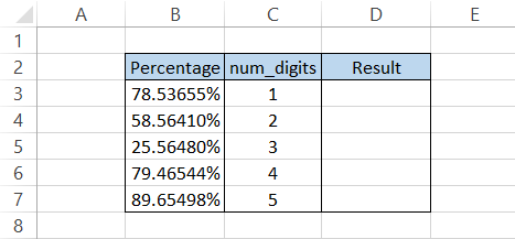
Using the formula =ROUNDUP(B3, C3), we will get the result:

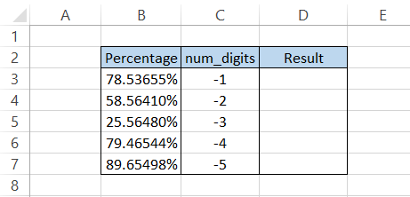
We believe by now, you can easily interpret the result that we obtain using the function. What do you think the effect of negative integers as num_digit argument would be?

Well, let's see!

Suppose the data in Excel is as illustrated below:

Using a similar formula, =ROUNDUP(B3, C3), we would get the result:

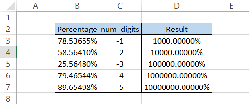
Whether the result returned is valid or not is up to you to decide where it could be helpful, but this is the effect of using negative integers as an input for the num_digits argument.

ROUNDUP vs. ROUNDDOWN Function

A ROUNDDOWN function works precisely opposite to its counterpart, i.e., it rounds up the numerical value towards zero. 

For example, if you have the number 78.53 and need to round down the value to just one digit after the decimal point, then using the function, you would get the result as 78.5.

On the other hand, a ROUNDUP function rounds the value away from zero, i.e., 78.53, to just one digit would become 78.6.

The syntax for the ROUNDDOWN function is:

=ROUNDDOWN(number,num_digits)

where,

• number = (required) the number which will be rounded to specified decimal places
• num_digits = (required) the number of decimal places that you want to round down the value 

Next, we will see an example to better understand both functions' differences.

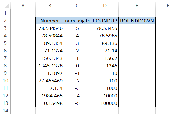
Suppose you have the data as illustrated below:

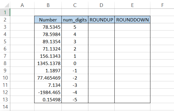
To find the result in column D, we will use the formula =ROUNDUP(B3,C3) and drag it down up to the last cell, which would give the result:

Similarly, to get the round down value in column E, we will use the formula =ROUNDDOWN(B3,C3) and drag it down to the last cell to get the result:

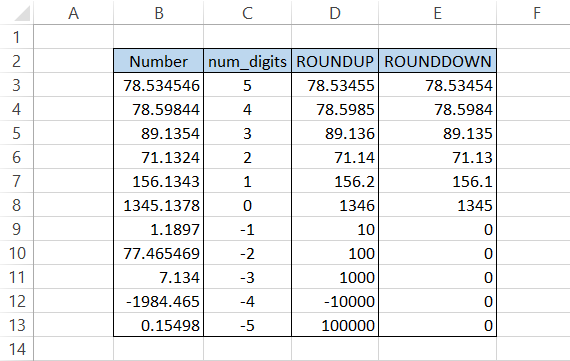
Even though both functions perform a similar task, i.e., rounding a value, they return quite contrasting results.

Researched and Authored by Akash Bagul | LinkedIn

Reviewed and edited by Parul Gupta | LinkedIn

Free Resources

To continue learning and advancing your career, check out these additional helpful WSO resources:

• MOD Function
• NOW Function in Excel
• PowerPoint Shortcut Keys
• REPLACE Function
• Scatter Plot