ABSOLUTE Function in Excel (ABS)

What is the ABSOLUTE Function in Excel (ABS)?

The Absolute or the ABS function in Excel returns the absolute value of a number.

Any given number can be positive or negative depending on the presence of the minus (-) sign before the number.

The function converts all the negative numbers into positive whereas the positive ones remain unaffected by the effect of the ABS function.

There are numerous situations wherein we write mathematical equations and expect a positive number. Instead, all we get is a negative number.

Instead of going through all the struggles of how the number can be returned positive, all you need to do is use the ABS function that converts any negative number into its positive counterpart.

This article will show the ABS function, its uses, and some examples.

Understanding Absolute Function In Excel

The ABS is categorized as a Math and Trigonometric function that returns the absolute value for a given number, i.e., it will return a positive number for a negative number.

If the function is used upon positive numbers, they remain unaffected. So, for example, if the number is 53 and you use the ABS function, the result will be 53.

However, if the number is -53 and the function is used, the expected result will be a positive 53. This is because the negative sign of the number automatically gets removed from the calculated value returning a positive number.

Apart from the sign change, there is no other effect on the given number.

The syntax for the function is

=ABS(number)

where

number - (required) the numerical value whose absolute value will be returned.

Example of Absolute function

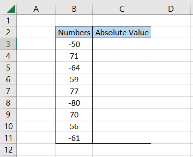
Give any number to the function, and it will return the absolute value within seconds. For example, suppose you have the numbers in Excel as illustrated below:

To use the function as a worksheet formula, we will begin with an equal sign, type in the function name, and add the cell reference inside the parentheses.

The formula in cell C3 will be =ABS(B3), which will be dragged down to cell C11 to give the result:

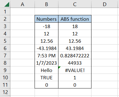
Interpretation:

1. When we have positive numbers, such as in the case of cells B4, B5, and B11, the result returned is a positive number.
2. A result is a positive number when the numbers are negative, as in cells B3 and B6.
3. When a text value is referenced in the function, Excel returns #VALUE! Error.
4. The boolean values TRUE and FALSE are stored as positive numbers. As a result, both ultimately return the same number.
5. Excel returns the same ‘positive’ serial numbers and decimal numbers counterparts for date and time values.

Practical Examples Of ABS Function

This section will show examples of using the absolute function in real-life scenarios.

a. Example #1

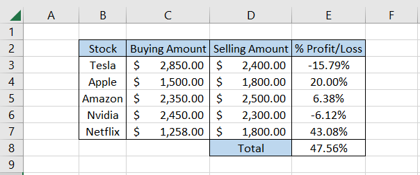
Suppose you invested in stocks by making a few trades. Then, after a year, you decide to redeem the capital by selling the stocks. The profit or loss earned on each transaction is represented below as a percentage:

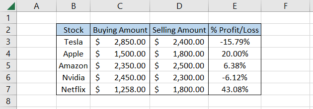
In this case, it makes sense to have a negative value for losses in column E. However, what if we still needed absolute values?

There could have been two ways: add a minus sign individually for all the negative values in column E so that they return a positive counterpart (remember, two negatives make a positive?) or use the absolute function.

It makes more sense to use the latter option since it gives faster results and saves you loads of time. Plus, it doesn’t interfere with the positive numbers, so it becomes the least of your worries.

By using the formula =ABS(E3) in cell F3 and dragging it down to cell F7, we get the result:

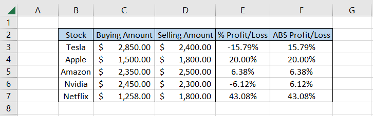
See? Same numbers, but without the negative sign. Netflix was the clear winner either way, but using the ABS function might make someone believe that Tesla made a profit of 15.79%.

b. Example #2

Okay, so we found the absolute percentage values. What if we wanted to skip this step and directly find the sum of ‘n’ positive and negative numbers?

For example, there are four numbers 1, 2, -1, and -2. We will get zero if we normally take the sum of those four numbers. However, Excel has a method to get the sum as absolute numbers.

Suppose you have the data as illustrated below:

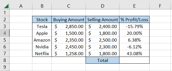
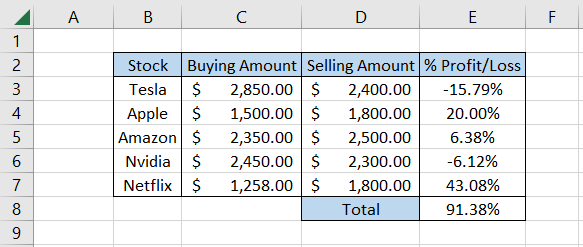
If we directly take the sum of the values in range E3:E7, we get the result as 47.56%, which might seem a bit misleading if we wanted the sum as absolute values.

Instead, we can use the combination of SUM and ABS functions to give the total sum of all the numbers in absolute terms.

The formula will be =SUM(ABS(E3:E7)) in cell E8, which gives you the result of 91.38%.

You do need to remember that since this is an array formula, you must press the Ctrl + Shift + Enter key on the keyboard, or else you will get the #VALUE! Error.

Thus, the combination of ABS and SUM functions enables you to directly get the ‘sum’ in absolute terms rather than returning individual absolute values and then calculating the total.

c. Example #3

So far, we have seen how to find the absolute values and how to directly find the sum of ‘n’ numbers in terms of their absolute values.

In this example, we will find the average of ‘n’ numbers in absolute terms.

Suppose the data is as illustrated below:

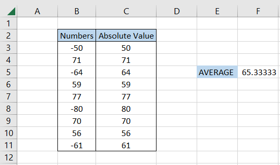
If we were to find the average of these numbers, the usual process would be to find the absolute values first and then calculate the mean value using the AVERAGE function.

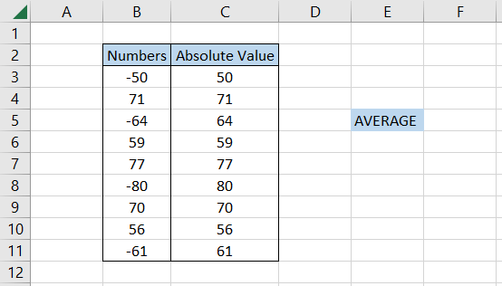
The formula in cell F5 will be =AVERAGE(C3:C11), giving the result 65.3333.

However, you can skip this entire process by using a simple formula =AVERAGE(ABS(B3:B11)) in cell F6, which gives the same result.

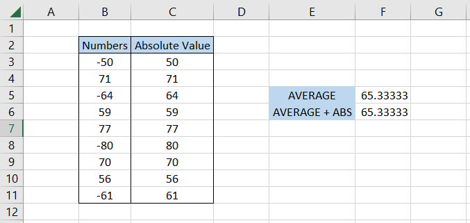
Similar to what we did with the SUM function, the combination removes the additional step of changing the values into their absolute counterpart.

Also, you need to press the Ctrl + Shift + Enter key since this is an array formula to get the correct result.

d. Example #4

Another way to use the absolute function is in combination with the TRUNC function.

The TRUNC function in Excel removes all the digits after a decimal point from the given numerical value. For example, if the number is 4.85, the function returns the result as 4.

Combining the TRUNC function with ABS makes it possible to extract the numbers after the decimal, even for the negative values.

Suppose the data looks as illustrated below:

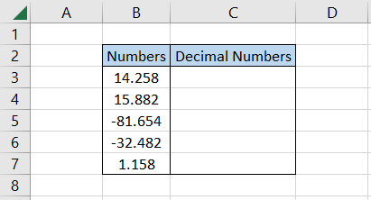
To extract only the decimal part, we will use the formula =ABS(B3-TRUNC(B3)) in cell C3 and drag it down to cell C7, which gives the result:

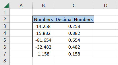
So, yes, even =B3-TRUNC(B3) would have been enough to get the decimal numbers.

However, using the ABS function helps us get the absolute numbers upon which we can perform different mathematical operations, such as finding the minimum and maximum values.

Researched and authored by Akash Bagul | LinkedIn

Reviewed and edited by Parul Gupta | LinkedIn

Free Resources

To continue learning and advancing your career, check out these additional helpful WSO resources:

• FIND Function
• Frequency function
• FV Function
• HOUR Function
• HYPERLINK Function