FIND Function
An Excel Text function that acts as a powerful tool utilized to search and return the position of a specific text or substring within a text string.


What is the FIND Function?
The FIND function is an Excel Text function that acts as a powerful tool utilized to search and return the position of a specific text or substring within a text string.
The FIND function is particularly helpful for distinct tasks related to text manipulation, data extractions, and conditional formatting.
In our daily lives, we are always looking for something, such as misplaced car keys, a late-night snack in the refrigerator, an excellent show to watch on Netflix or the love of our life.
Generally, people are always searching for something related to their lives. In such situations, when there is someone to guide us, the task becomes much more accessible.
I can count all the instances when the car key was lying precisely in front of me, and yet I couldn't find it until I got my Mom's instructions: "Top shelf near the TV."
Excel's FIND function works similarly. It looks for something based on your guidance and returns its exact position.
When you input a text string or a string of numbers, the function can return a character or a substring inside that text string.
The function is rarely used alone; combining it with other text functions, such as LEFT, RIGHT, and MID parts, enables you to extract characters based on their position in the text string.
This article will guide you through the syntax of the function and provide examples of how to use the process to extract data from a string of characters.
- The FIND function returns the position of a substring within another text string based on predefined conditions.
- The FIND function returns the position of find_text within within_text, starting from the first character of within_text as position 1.
- FIND is case-sensitive, distinguishing between uppercase and lowercase letters. If find_text is not found within within_text, FIND returns the #VALUE! error.
- FIND is useful for extracting data from strings, such as parsing addresses, names, or other structured data. It can also be used to locate specific characters or words within larger text strings.
Understanding The FIND function
The FIND function is a text function that returns the position of a substring or a character inside another text string.
For example, if you have the text string as 'Americans have an average credit card debt of $6,270' and need to search the position for the substring 'credit' in the text string, then the function will give the result as 27.
The function begins counting the characters from the left-hand side and returns the position as a number corresponding to the first letter of our substring.
Even though our substring' credit' has six characters in total, the function only focuses on the first character 'c' and returns its position that agrees with the entire substring.
The function is very similar to the SEARCH function, which also returns the position of a string of characters from another text string. The only significant difference between both functions is that SEARCH is case-insensitive and allows the use of wildcards.
For example, if you have the text string 'Tesla Inc' and ask the function to search for the position of 'Tesla,' it will return a #VALUE! Error.
If you need to search for something in a text string, you must be precisely specific, including capitalized and lowercase letters. In the case of the SEARCH function, you wouldn't face the exact match problem.
On the other hand, if you look for a wildcard + substring "Tes*" using the SEARCH function, it will return the result as 'Tesla.' However, you would get the #VALUE! Error in the case of its counterpart.
FIND function Formula
The syntax for the function is:
=FIND(find_text, within_text,[start_num])
Where,
- find_text = (required) the substring we intend to search in a text string.
- within_text = (required) the text string which will be searched for the substring
- start_num = (optional) the starting position to search the character or substring in the within_text argument. For example, the text string 'Hello' consists of five symbols. Therefore, we need to look for the position of second 'l.'
If we use the start_num argument either as 1,2, or 3, we will get the position only for the first 'l.' However, when we use the start_num as 4, we get the result as the second 'l' present in the text string.
The argument signifies the starting position from which the characters will be counted to search the part of our target substring.
Thus, the start_num argument can be beneficial in skipping a certain number of characters if they are repetitive and return the desired substring immediately as per convenience.

How to use the FIND Function in Excel?
The function can be used from the library or a worksheet formula. We will see both methods, and you can decide which method best suits you.
Method 1: From the library function
If you aren't good with the formulas, the function should be your go-to tool. Parts already have the rules set up and precisely guide you on what arguments need input to get the required result.
First, select the cell in which you need the result.

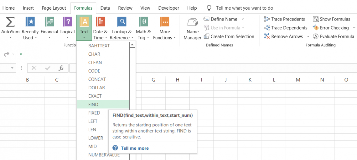
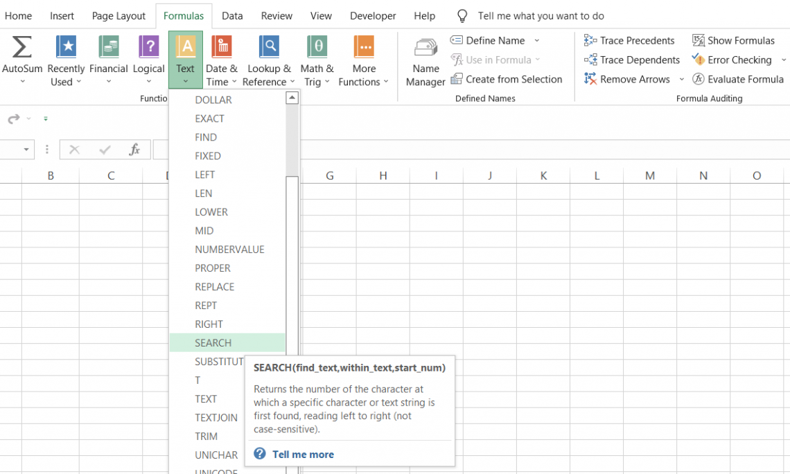
Click on the Formulas tab > Text drop-down on the function's library and select the FIND function.
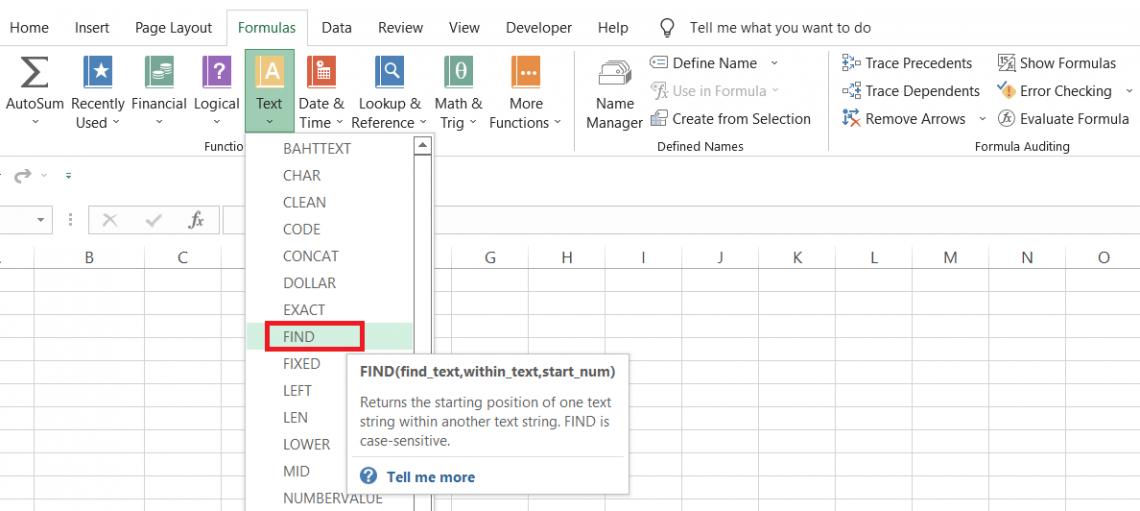
This will open up the dialog box, as illustrated below:
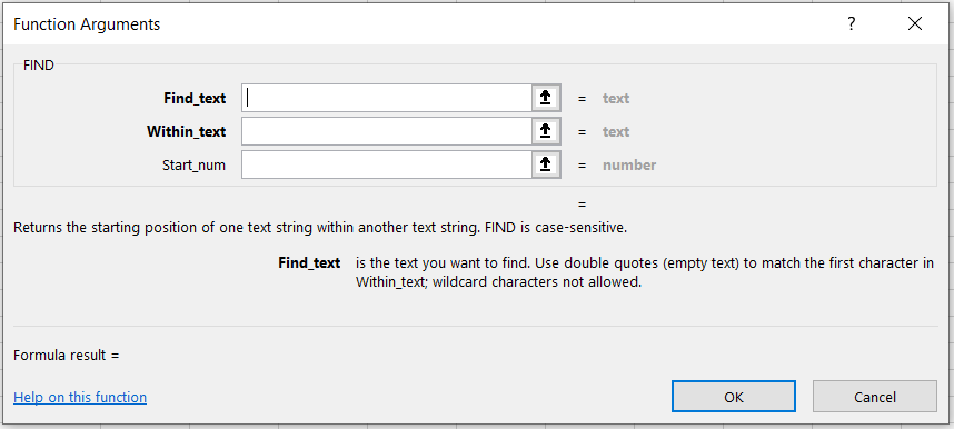
Input the arguments in the respective text boxes as per the function's syntax. For example, we have input the ideas below:
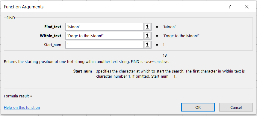
When you click on OK, you will get the following result:
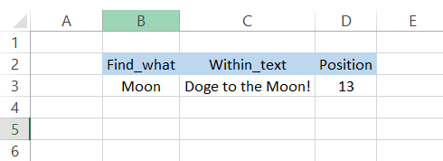
If we press F2 in the D3 cell, we see that it is a =FIND("Moon," "Doge to the Moon!",1) formula.
Since 'M' is the starting letter for the substring 'Moon,' Excel counts up to that character and returns its position corresponding to the entire substring.
The start_num argument as 1 counts from the first character beginning from the left-hand side.
Method 2: From the library function
The function can also be used as a worksheet formula where you begin with an equal sign(=), followed by the formula name and the arguments inside the parenthesis.
Suppose that you have the text string as illustrated below:
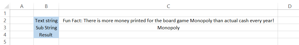
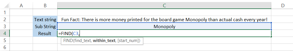
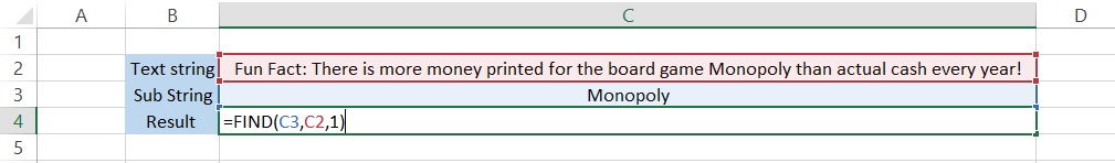
find_text - The text we intend to search is in cell C3. The formula becomes =FIND(C3,within_text,[start_num]).
within_text - Next, we reference the cell where we intend to look for the substring present in cell C2. The updated formula becomes =FIND(C3,C2,[start_num]).
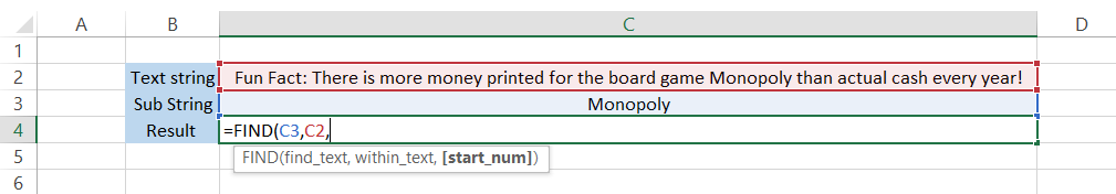
start_num - Finally, we input the argument for the optional parameter or can skip it, which assigns it a default value of 1. To be precise, we use the 1 as the start_num and the closing parenthesis.
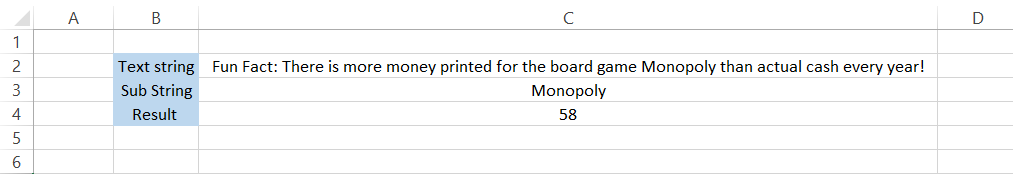
Once you press Enter, you will get the substring 'Monopoly' position as 58.
We know the FIND function is case-sensitive, so what would the result be if we reference lowercase 'monopoly' instead of 'Monopoly'?
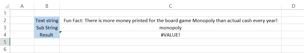
We get a #VALUE Error since Excel cannot search our substring beginning with a lowercase 'm'. Thus, you must be precise when searching for something using the function.

FIND Function Examples
In this section, we will see examples to better understand the function.
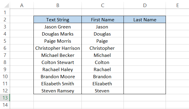
Example 1: Separating first and last name
Suppose you must extract the first and last names from the full terms.
The data looks as illustrated below:
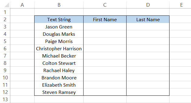
To get the First Name, we will use the combination of the LEFT and FIND functions so that the formula is =LEFT(B3, FIND("",B3,1)), which will give you the result:
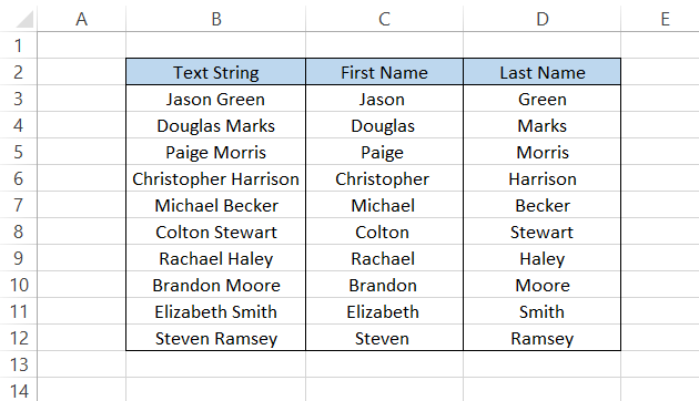
Similarly, to search the last name, you can use the combination of RIGHT, LEN, and FIND functions so that the formula becomes,
=RIGHT(B3,LEN(B3)-SEARCH(" ",B3,1))
It should give you the required result in column D.
There are a lot of different text manipulation formulas that you can use to extract a particular substring based on the delimiter present in the text string.
A delimiter is a character, such as a space or an asterisk, that separates text by forming a boundary between them.
Example 2: Check for the presence of a string
The function works wonders if you need to check for the presence of a particular substring in the main text string.
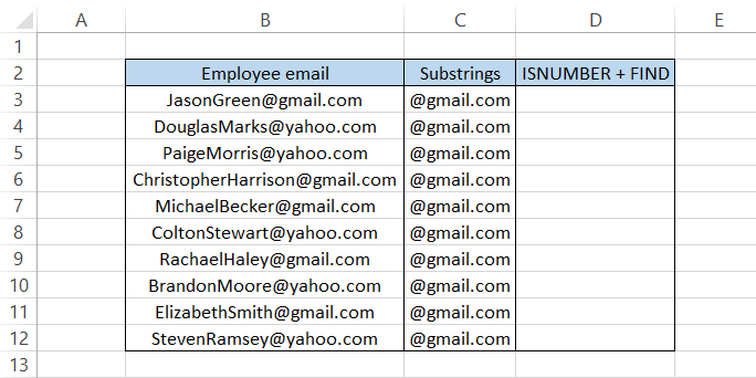
You can use the combination of functions ISNUMBER and FIND to check whether all the email IDs have the domain name @gmail.com.
The formula will be,
=ISNUMBER(FIND(C3,B3,1))
It should give you the result, as illustrated below:
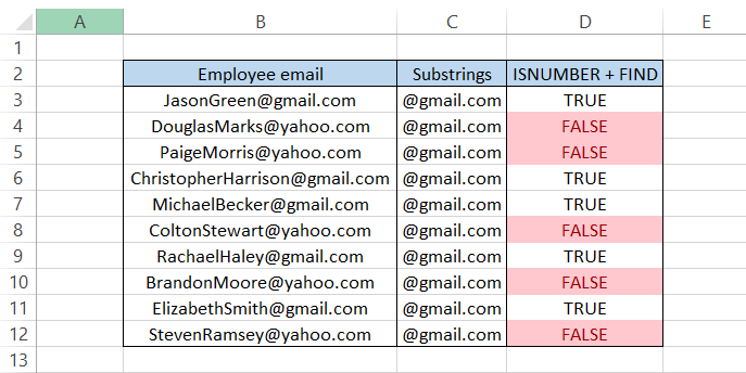
If the substring exists in the employee email, the function will return the position of that substring as a numerical value.
The same numerical value is then passed to the ISNUMBER function, which evaluates the result to TRUE or FALSE.
Example 3 - Extracting text up to the 'nth' term
In one of our previous examples, you saw how to separate the first and last name based on the presence of a delimiter 'space' character.
We will use the same concept to extract a text up to the nth term. For example, if a sentence consists of 10 words and we need to remove only up to the 8th term, the combination of LEFT, FIND, and SUBSTITUTE functions.
Suppose that we have the text string in cell C3, as illustrated below:
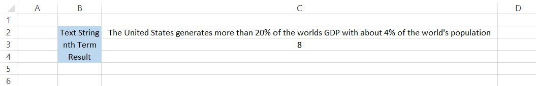
To get the text string up to the 8th word, we will use the formula,
=LEFT(C2,FIND("@",SUBSTITUTE(C2," ","@",C3))-1)
It will give the result in cell C4 as follows:
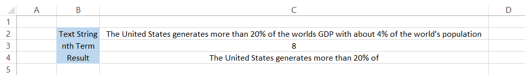
In our result, each substring separated by a delimiter 'space' character is counted as one word.
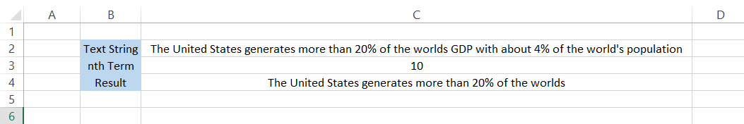
If we change the nth term to 10, the result changes and returns a text string consisting of 10 words separated by 9 space characters.
To understand the formula better, we will try to break it down into the three constituent functions used.
- SUBSTITUTE function - The function nested in innermost has a simple task of replacing all the 'nth' space characters with another character such as '@.' As a result, if the nth term is 2 and the text string is 'Welcome to WallStreetOasis,' the resulting line would be 'Welcome to@WallStreetOasis.' The rest of the space characters remain unaffected by the effect of the SUBSTITUTE function.
- FIND function - The function then searches for the '@' character in the text string. If found, the character's position is returned as a numerical value.
- LEFT function - Finally, the LEFT part takes that numerical value as a num_chars argument and extracts our resultant text string.
FIND vs. SEARCH function
The SEARCH function in Excel is categorized as a text function that looks for a particular substring and returns its relative position in a text string.
Both functions work the same way, but the only significant difference is that the SEARCH function is case-insensitive.
For example, if you need to look for 'A' in 'Apple,' the character we are searching for could be 'a' or 'A,' and we still would get the answer, unlike the FIND function.
It doesn't matter whether all the letters are lower or uppercase, but if a similar match exists in the text string, the function will return its relative position.
The syntax for the function is
=SEARCH(find_text,within_text,[start_num])
Where,
- find_text = (required) the substring we intend to search for in a text string.
- within_text = (required) the text string that will be searched for the substring.
- start_num = (optional) the starting position within the text string.
While the SEARCH function offers more extensive flexibility in looking at the position of various substrings, its counterpart provides the chance to improve the precision of looking for a substring. Hence, both functions have their pros and cons.
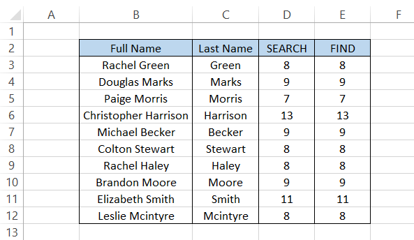
Suppose that you have the data in Excel, as illustrated below:
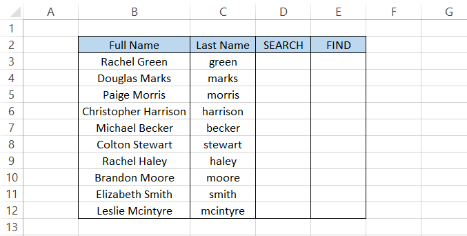
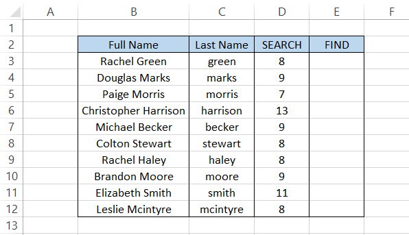
We need to look for the positions of the last names in the text string. To get the job using the SEARCH function, we will use the formula =SEARCH(C3,B3,1), which should give the result.
In the same way, if we use a similar formula, =FIND(C3, B3,1), we fail to get the result and instead get the #VALUE! Error.
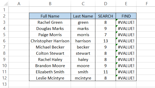
Only when the substrings in column C match precisely that in the text string can the function return the position using both processes.
On the other hand, when you make the changes, there is no effect on the result for the SEARCH function. Thus, using either part can be an advantage or a disadvantage to the user as per the working scenario.
Another reason the SEARCH function might be superior to its counterpart is its ability to search substrings based on wildcard characters.
By using a few characters followed by a wildcard, such as an apostrophe(*), you can let Excel decide whether to base the result on the available alternatives.
For example, if you use the substring "He*," Excel will return possible results such as 'Hello,' 'Hell,' 'Hey,' etc., based on their availability.
Suppose you must extract the substring that matches the word 'pop.' The main text string that will be searched for is:
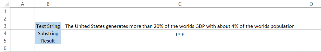
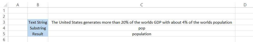
To extract the word that matches our substring, we will use the formula,
=MID(C3,SEARCH(C4&"*",C3,1),LEN(C3))
The result obtained in cell C5 is:
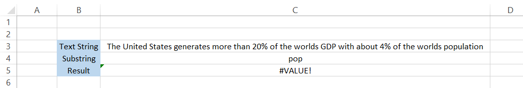
If you substitute the SEARCH function with FIND by using the formula
=MID(C3,FIND(C4& "*",C3,1),LEN(C3)), you wouldn't get the same answer since it does not support the use of wildcard characters.
Instead, Excel throws in #VALUE Error to us.
Free Resources
To continue learning and advancing your career, check out these additional helpful WSO resources:


or Want to Sign up with your social account?