ISERROR Function
Helps a user identify any errors occurring in calculation, value, string, reference, etc.


What is the ISERROR Excel Function?
Suppose you have an important Excel spreadsheet to prepare, which involves vast calculations and number crunching.

Also, you want no error or mistake must occur which might impact your spreadsheet. To ensure this, Excel helps us by making us aware of any errors during the calculations. This can be effectively implemented by using the ISERROR function.
This is an Excel function that helps a user identify any errors occurring in calculation, value, string, reference, etc. Of course, humans make errors, but this Excel function allows for catching such errors.
Like every other Excel function, this function acts on data by taking arguments and returning TRUE, FALSE, or any additional value as specified when used with the IF function.
In simple and default terms, you will get TRUE or FALSE if the calculation contains any error.
You will get TRUE if there are no errors and FALSE if there is any error. We will further discuss the different types of mistakes this function returns.
As discussed above, we can also return any other value specified in its formula or a message as per the user. It is combined with the IF function, VLOOKUP function, etc.
Types of Errors
Before we use the function, we need to understand the types of errors it usually catches and can act upon.
We have broken down the types of errors as under.
Everyone makes errors, and humans operating MS Excel make errors now and then; these errors have different types.
This function identifies such errors and reports them to you. Some of the widely witnessed errors are listed here:
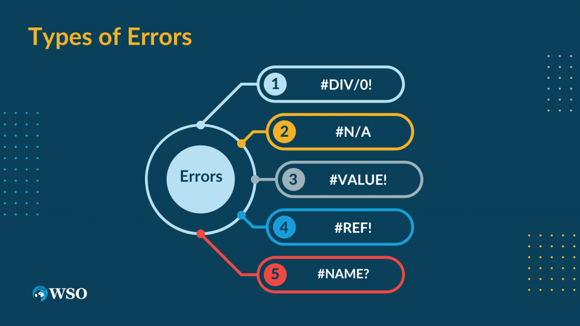
1. #DIV/0!
Suppose you are dividing two numbers, and by mistake, you have put 0 instead of 9, so the answer is not defined mathematically. But Excel will tell you such an error as #DIV/0.which means division by zero is not possible.
2. #N/A
N/A means “not available.” This error says it cannot find the value it needs to return. This happens when the formula references a cell or range that does not possess any value.
3. #VALUE!
Suppose you are referencing your cell to a number format cell but mistakenly referenced the formula to a cell that does not contain a number but text.
Excel will return this error, pointing out to the user that the format of the value that had to be referenced is not of such format.
4. #REF!
Such an error usually occurs when a formula references a cell or a range that does not exist, or we can say that we had previously deleted such a cell or range.
A reference error occurs when the user mistakenly refers the formulas to a deleted cell.
5. #NAME?
Name error usually occurs when the formula references an incorrect cell, the arguments of the formula are incorrect, the formula is incorrect, or the sequence of the arguments in the formula is wrong.
Components of the ISERROR function
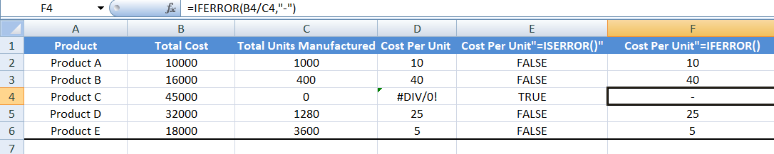
Suppose you have to calculate the quotient, which is possible by dividing the numerator(total cost) by the denominator(Total Units Manufactured).

In the following example, we have divided the Total cost by the Total units Manufactured. Usually, it will look like this without using this formula:
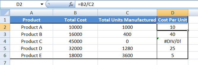
If any error occurs, suppose there are zero denominators, the answer will be #DIV/0! Error can be substituted by TRUE or FALSE to check whether such an error exists in our spreadsheet.
The syntax is described below, also with an explanation:
=ISERROR(A2/B2)
By using this formula, you can get TRUE or FALSE. When there is an error, the result is TRUE and FALSE when no error exists.
The syntax of the function is
=ISERROR(Value)
where
Value = any argument; it could be numeric or any expression that needs testing.
The returning value of this function is either TRUE or FALSE.

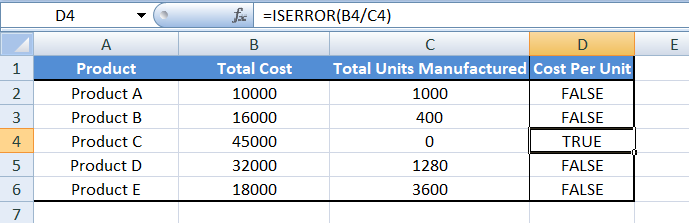
ISERROR and IF Function
Usually, the ISERROR function is used with the IF function. Using this function in combination with the IF function will help us to return a value as specified by the user and not the syntax of any of the above-listed errors.

The ISERROR function allows users to check a formula for any error and then returns TRUE or FALSE.
This means it does not allow the user to return anything other than TRUE or FALSE. But, to facilitate its resolution, one can use the IF function accompanied by the ISERROR function. This can help a user return a user-specified message, a string, or anything else.
This means we need to nest the IF function with the ISERROR function.
The IF function has the following arguments implemented with this function as its logical argument.

Where the IF function tests the condition in the ISERROR Function.
The condition that will be tested is if the result is TRUE, it returns the value for the following argument; if false, it returns the value for the end argument.
=IF(ISERROR(main_formula()), text_or_calculation_if_error_occurred, formula_for_normal_ result())
Where the IF function tests the first condition, if it becomes TRUE, the text or calculation will be displayed, and if the condition becomes FALSE, it will show the normal result.
ISERROR is a true-false function, and it delivers TRUE or FALSE for the logical test of the IF function.
A message can be displayed when the logical test becomes TRUE, meaning an error exists. If false, the logical test can be shown as a whole.
ISERROR vs. IFERROR
We have covered ISERROR and its utilization with the IF function. Now we are going to draw a comparison between ISERROR and IFERROR.

Suppose we don't want to use the IF function, but we also want to show a user-defined message if any error occurs.
This can be done effectively by implementing the IFERROR formula.
IFERROR function helps catch any errors present and also helps in returning a value if there is some error.
It can catch all types of errors; hence this function is an upgrade of the ISERROR function, as it delivers a message, any numeric expression, etc.
The syntax of the two can draw out a significant comparison of their features:
=IFERROR(value, value_if_error)
=ISERROR(value)
The value of the IFERROR is derived through a process similar to the ISERROR.
Suppose a user enters a value in the IFERROR formula and a value if error. First, it will check whether the value is an error, i.e., TRUE or FALSE. If it is True, the value_if_error is shown in the cell, and the value if False will show the value in the first place.
Hence, it is a privilege for the IFERROR function over the ISERROR.
ISERROR is an information function, and IFERROR is a logical function of MS Excel.
IFERROR can also be used with functions such as IF, VLOOKUP, INDEX MATCH, SUMPRODUCT, etc.
NOTE
The IFERROR function is much superior as it also provides a way to input any text or calculation if there is an error.
ISERROR vs. ISERR
People often confuse it with what function to use, ISERROR or ISERR. As far as we have discussed the way ISERROR works and the different combinations it works with. We will now discuss the ISERR function and compare the two with each other.

ISERR function is the same as ISERROR, but the only difference is that it does not catch any #N/A error.
Yes, you read it right. It does everything and can be used like the ISERROR function, but it cannot identify any #N/A error.
ISERR returns TRUE or FALSE depending upon any error in a numeric operation or expression.
The syntax for ISERR is as follows:
=ISERR(value)
The Excel Iserr function tests if an initial supplied expression (or value) returns any Excel Error, except the #N/A error. If so, the function returns the logical value TRUE; if the supplied value is not an error or is the #N/A error, the ISERR function returns FALSE.
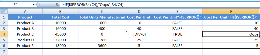
In the following example, we will see ISERR works.
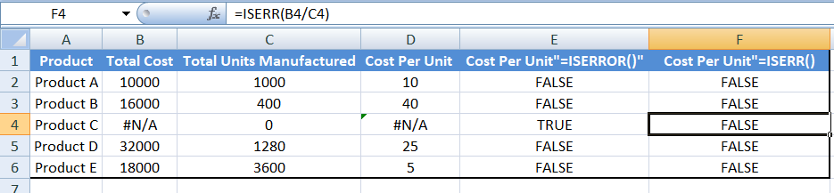
In cell F4, it can be seen that the ISERR function has returned FALSE; on the other hand, the ISERROR function has returned TRUE.
It can be interpreted that the ISERR function has worked on every data and every type of error but couldn't identify an #N/A error and has returned FALSE, showcasing there is no error. However, there is an error that ISERROR placed.
NOTE
ISERR function catches every type of error, not the #N/A errors.
ISERROR to count the number of errors
If we want to count the total number of errors in our spreadsheet, we use the SUMPRODUCT function accompanied by the ISERROR function. The syntax for the formula will be:

We generally use the double unary operator(--) to convert the TRUE and FALSE to 1s and 0s.
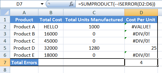
In this example, we have messed up with the earlier present number to show the calculation of the total number of errors.
In cell D4, we have calculated the number of errors. As ISERROR counts all types of errors, it has counted four in the various rows.
We can get the same result if we use the SUM function. Using the double unary operator, we can turn the TRUE or FALSE to 1 and 0, which the SUM function will count and give the sum of such numbers, which will be the total number of errors in the spreadsheet.
The formula for this is as follows:
=SUM(IF(ISERROR(cell range), 1, 0))
In this formula, we have converted the TRUE or FALSE to 1 or 0 with the help of the IF function.
Then the sum function will be able to calculate the total number of 1s and 0s and give the correct answer.
NOTE
The SUMPRODUCT function, accompanied by the ISERROR function, helps count the number of errors in a particular cell/range.
ISERROR and Conditional Formatting
Conditional formatting is an MS Excel feature that helps us format those cells or ranges that do not fulfill a specific condition mentioned.

For Example- A cell color will turn green if the value is >100.
Steps:
- Select the cell range which needs to be formatted conditionally.
- Click the Conditional Formatting button on the Excel Ribbon in the home tab.
- Select New Rule from the drop-down.
- A dialog box will appear where the user can select and use a formula to determine cells to format.
- Enter the formula below as =ISERROR(cell range).
- Choose the format you want the cells to have an error appear.
- Click OK.
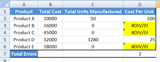
This tool is helpful because it can help make the user aware of the errors made in the spreadsheet by highlighting such erroneous cells and making it easier for the user to reduce errors.
NOTE
When used with this function, conditional formatting will yield great results, which help identify and catch errors. This is done by highlighting the cells which contain an error.
Troubleshooting and ISERROR function
Generally, when using this function, we may encounter an error or errors we didn't expect to occur.

In this section, we will provide fantastic tips to help make your spreadsheet error-free by using the following troubleshooting tips.
1. Check your data format.
The function works with numeric and text data, so you must personally ensure that the data format is per your needs and must be one of the two mentioned.
Suppose you have used a date or a boolean value (True/False). You will be making an unexpected error.
2. Check the Syntax
Always remember to triple-check that you have used the correct syntax. Syntax is a way of writing commands.
You need to check through these commands to see whether they are correct or if there are any discrepancies in the syntax, such as spelling or incorrect arguments.
3. Proper use of Parentheses
When we are performing the nesting functions or using the ISERROR function with other functions, it must be ensured that the parentheses are in the correct position, and there must be the right number of parentheses.

Excel usually points out if there is any discrepancy in the position of the parentheses or their number, and the user needs to click OK to accept changes.
When you click OK Excel, you might think of the correct argument different from the user's needs, which may lead to an unexpected error.
4. Test individual components
One can also test each formula element separately if facing an error.
For Example- If you are trying to count the total number of errors with ISERROR and getting a mistake, you can use the COUNTIF function with the condition "not equal to #N/A!". This will help to count the total non-erroneous cells.


or Want to Sign up with your social account?