MID Function

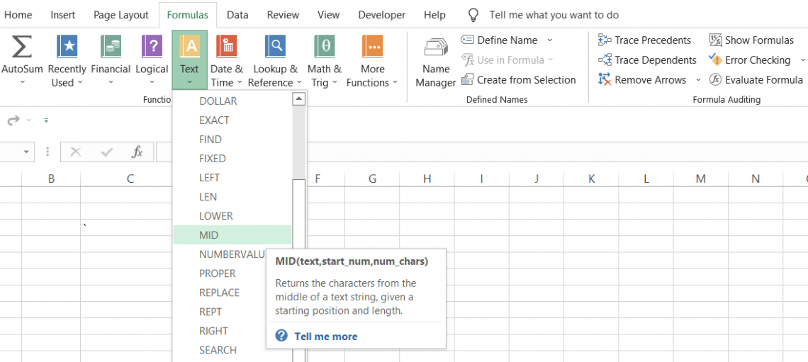
What is the MID Function?

The MID function in Excel extracts the 'n' number of characters from the middle portion of a text string. Excel has grown from a number-crunching tool to a more sophisticated reporting instrument.

Since the gridlines make distinguishing between two or more cells easier, most organizations prefer to create reports in Excel rather than MS Word or any other software.

For example, operational due diligence reports are often submitted by companies to report their business models and operations targets of the company. However, if you ever come across such messages, you would find that more than 80% of data is textual while only 20% numbers.

And yet, those reports are prepared in Excel!

Even after 35+ years, Excel has been the go-to tool for all financial analysis and data handling.

And even though the MID function is just a speck of dust in the entire Excel universe, it has enough capability to create a rippling effect amongst the Excel community to portray the function's importance.

Understanding MID function

The MID function is categorized as a text function that will extract specific numbers of characters from a text string.

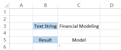
For example, if you have the text string as 'Financial Modeling,' you can extract the 'Model' part while trimming away the unnecessary characters from the text string.

First, you must reference the text string or directly hardcode it into the formula to use the function. 

Next, you describe the location of the first character that you intend to extract. 

For example, in our model, the first character we wanted to pull was the letter M, which holds the 11th position in the text string. Always remember that even a space character takes up an additional character.

The last parameter expresses how many characters you need to draw out. For example, if we input 5 as our argument, the function should return exactly five symbols from our beginning location, which gives the word 'Model.'

As we said, even though the function looks like it doesn't show much potential. But believe us, once you understand what it is capable of, it will be one of your favorite functions for text strings.

MID Function Formula

The syntax for the function is:

=MID(text, start_num, num_chars)

where,

• text = (required) The text string from which you intend to extract the characters
• start_num = (required) the position of the first character in the text
• num_chars = (optional) the number of characters to extract from the text. If you skip the argument, the function takes in the default value of 1

How to use the MID Function in Excel?

Let's begin with a simple model and build up from that to see just how valuable the MID function can be in your day-to-day life while working on data.

Example 1

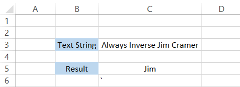
Suppose that you have the text 'Always inverse Jim Cramer' in the spreadsheet, as illustrated below:

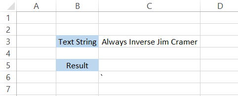
Let's say we want to pull out the word 'Jim' in cell C5. We can see it is a 3 letter word, so we are clear about the value for argument num_chars.

However, to find the starting position, we need to count the number of characters beginning with the letter A as 1. Also, don't forget to count the spaces, as they are also considered Excel characters.

After counting the characters up to the letter' J,' we find its position is 16th in the text string.

Since we have all our arguments now, we will use the formula =MID(C3,16,3), giving you the result as 'Jim' in cell C5.

Example 2

As a financial analyst, the texts you see are first and last names. However, you will always have reports with borrower names if you work in a bank or an Asset Management company.

With these reports, there could be instances when you need to separate the first name and last name of the borrower. 

For example, the full name might be separated by an unwanted character such as underscore(_), which won't be accepted by your database and hence needs to be separated.

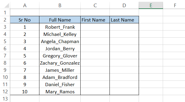
In such a case, you can use the combination of MID and SEARCH functions to separate the first and last names. For example, suppose the data looks as illustrated below:

We will use the formula =MID(B3,1,SEARCH("_",B3,2)-1) in cell C3, which will give you the result as 'Robert'. Drag down the formula till the cell C12, and the spreadsheet should look as:

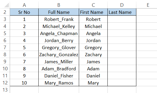
By subtracting 1, we remove an additional character from the string that is returned as a result, or else the expected text string would be 'Robert_' in cell C3.

We will use a similar formula to get the last name, but it will include an additional LEN function.

The formula that we will use will be =MID(B3, SEARCH("_," B3,1)+1, LEN(B3)), which should give you the result in cell D3 as:

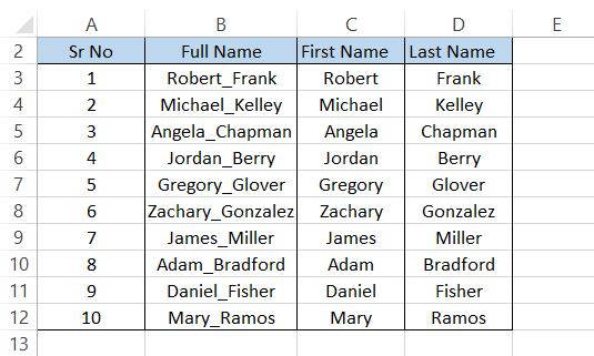
Just like you need to balance the assets and liabilities on a balance sheet, here we have added 1 to remove the additional character from the string to avoid getting the result as '_Frank.'

Since most surnames have a varying character count, it wasn't feasible to hardcode a numerical value to return the number of characters.

There is an option to just hardcode a significant number, say 1000, but we want our formulas to be dynamic. Hence, we have included the LEN function that will automatically capture the length of the string and, thus, extract the last name.

Example 3

The function can also help extract a text string between two 'delimiters.' For example, 'New York(NY)' is separated by a comma on both sides, thus limiting and forming a fictitious cage worldwide.

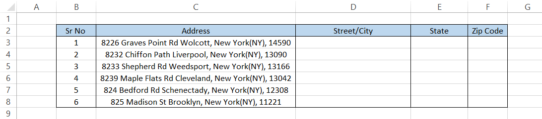
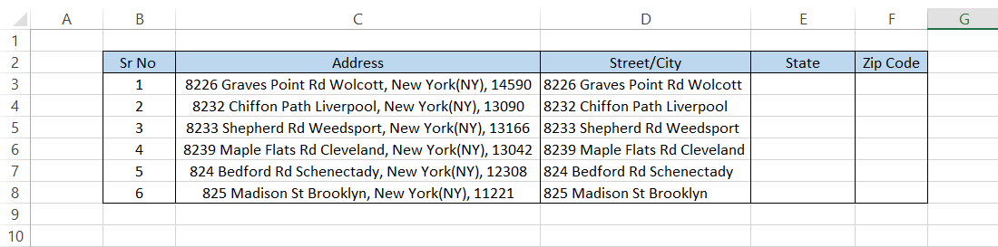
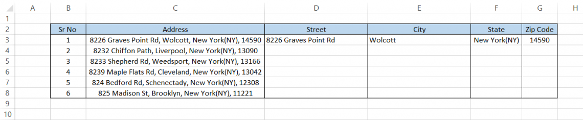
Suppose that your bank intends to lend loans to some of the borrowers. The documents are filed, and the records are set up on the primary database. 

However, the admin department fills in the address in one single line as ‘8226 Graves Point Rd Wolcott, New York(NY),14590'.

This isn't a problem, but another team of your bank analyzes these addresses and, based on the zip codes, determines what area has a higher loan demand and strategizes their goals accordingly. 

The data for the address looks as illustrated below:

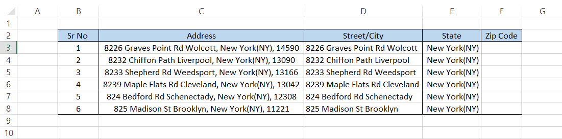
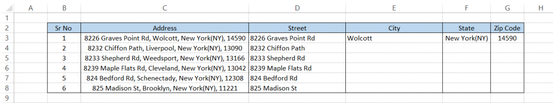
To extract the street and city, we will use the formula =MID(C3,1, SEARCH(",", C3)-1), which will give you the result ‘8226 Graves Point Rd Wolcott' in cell D3.

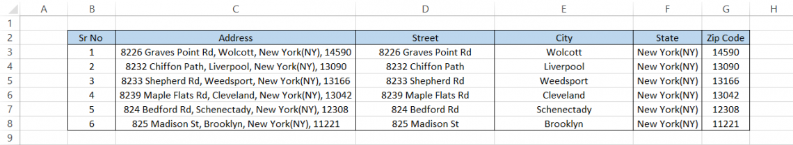
Similarly for state we will use the formula =MID(C3,SEARCH(",",C3,1)+1,SEARCH(",",C3,SEARCH(",",C3)+1)-SEARCH(",",C3)-1), which should give you the result as:

For the zip code, we won't be using the MID function but rather the RIGHT part using the formula =RIGHT(C3,5), which will only extract the zip codes from the text string.

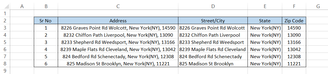
This data can now be passed onto the central database so the analytics team can work and determine the neighborhood with potential loan borrowers.

We hope you understand how the MID function works through these' examples.' But now I'm about to end this function's whole career.

MID Function Alternatives

We all have heard of the flash fills now and then. Unfortunately, although it is relatively elementary, many people are unaware of using flash serves in Excel.

Suppose we have the same address in Excel as illustrated below:

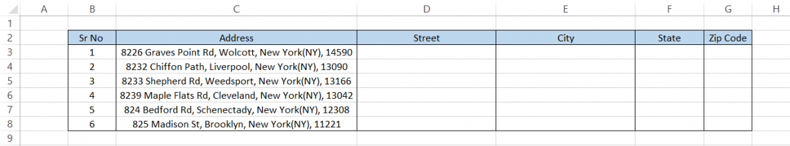
A minor change we have made in our address is adding a 'delimiter' in the form of a comma before the city so that both elements are separated.

Our first step is to write the text we want to return in our respective columns. For example, for the street, we need only ‘8226 Graves Rd'; for the city, it would be 'Wolcott,' while the state and zip code will be 'New York(NY)' and '14590,' respectively.

All of these would be hardcoded in individual cells, which will look as illustrated below:

The next step is to head to cell D2 and press the combination of Ctrl + E. And voila! In just a second, Excel separates all the streets in column D.

Similarly, the rest of the data can be pulled in using the magic key combination of Ctrl + E. In just a few seconds, you will get the entire data separated, as illustrated below:

So yes, if you have a 'delimiter' between the data you intend to separate, Flash fill is the best option if you aren't good with formulas. But if that's not the case, the good ol' MID function would do the job.

If you aren't yet ready for our Excel Modeling Course, we hope you enroll in our Excel Crash Course, which is a foundational course for IB+PE and will get you on track with some of the Excel functions you aren't familiar with! 

MID Function Practical Example

Let's take a look at a practical example of the function below:

Practical Example - Finding the nth word in a sentence

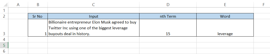
Suppose that you have a text string and need to find the position of a specific word within the sentence. How can you find, let's say, what the 10th word is?

Suppose that the text string in Excel is as illustrated below:

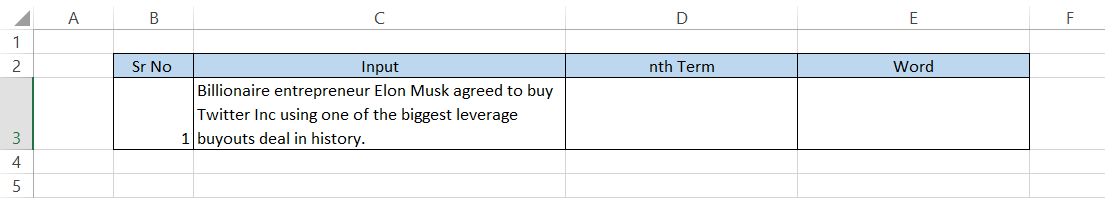
You will use MID, TRIM, SUBSTITUTE, LEN, and REPT functions to find the nth term.

You might know how other functions work, but REPT might be relatively new to you. 

The function repeats a given character 'n' several times.

The formula that you will use is =TRIM(MID(SUBSTITUTE(B3," ",REPT(" ",LEN(B3))), (C3-1)*LEN(B3)+1, LEN(B$3))), which will give you the result as below:

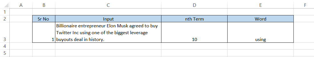
As you change the nth term in cell D3, the result in cell E3 changes. For example, if the nth term is15, the formula will return the word as 'leverage'.

So how does the formula work? Let's break it down into steps:

• Firstly, the LEN function finds the string's length equal to 121 characters
• Next is the use of the REPT function, wherein the formula REPT("", LEN(C3)) gives us a total of 121 spaces
• The formula =SUBSTITUTE(C3," ", REPT("", LEN(C3))) will replace all the space between two adjacent words with spaces equal to 121
• The result is then enclosed inside the MID function that returns the word based on start_num(the beginning position) and the num_chars(number of characters to extract)
  Our start_num will be (D3-1)*LEN(C3)+1, where the logic is that each word is separated by 121 spaces, i.e., Billionaire + 121 spaces + entrepreneur, wherein the start_num directly lands us on our next word in sequence
• The formula so far is MID(SUBSTITUTE(C$3," ",REPT(" ",LEN(C$3))), (D3-1)*LEN(C$3)+1, LEN(C$3))
• Even if the word is extracted, we don't have to forget about any additional spaces that the formula might return in the result

Hence, we will use the TRIM function, i.e., =TRIM(MID(SUBSTITUTE(C$3," ", REPT("", LEN(C$3))), (D3-1)*LEN(C$3)+1, LEN(C$3))), such that it removes all the additional spaces from the text, which finally returns the word based on the nth term that you input in cell D3

Researched and authored by Akash Bagul | LinkedIn

Reviewed and edited by Parul Gupta | LinkedIn

Free Resources

To continue learning and advancing your career, check out these additional helpful WSO resources:

• FV Function
• PEARSON Function
• SEARCH Function
• SUBTOTAL Function
• YIELD Function