MOD Function
Returns the remainder for two numbers, i.e., a dividend and a divisor


What is the MOD Function?
MOD is categorized as a Math & Trigonometric function that returns a remainder based on two numbers wherein one is a dividend, and another number is a divisor.
The MOD function in Excel returns the remainder for two numbers, i.e., a dividend and a divisor.
You might vaguely remember your math classroom in childhood. If there were still memories of two mathematical concepts, then it is the relationship between the dividend-divisor and the calculation of LCM.
The function is largely based on the former mathematical relationship and helps to find the remainder based on two different numbers.
The same concept holds significant importance in real-life scenarios, so Excel had to devise a function that would suffice this particular need. And the function is none other than MOD.
As a kid, we always had this confusion regarding dividends and divisors. What gets divided by what? The confusion has stayed all these years, so we will take a few seconds to explain both numbers.
The dividend will be the number in the numerator which will be divided by the divisor in the denominator.
For example, if the dividend is 10 and the divisor is 7, the remainder for the two numbers will be 3.
Generally, if we take divisions 10 and 7, the result should have been 1.42857. However, the very concept here is to return a remainder that will only be zero when the dividend is perfectly divisible by the divisor.
For example, if the number is 15 and the divisor is 5, then in this case, the result will be equal to zero.
This article will guide you on the function and how to make the best use of it, along with a couple of examples

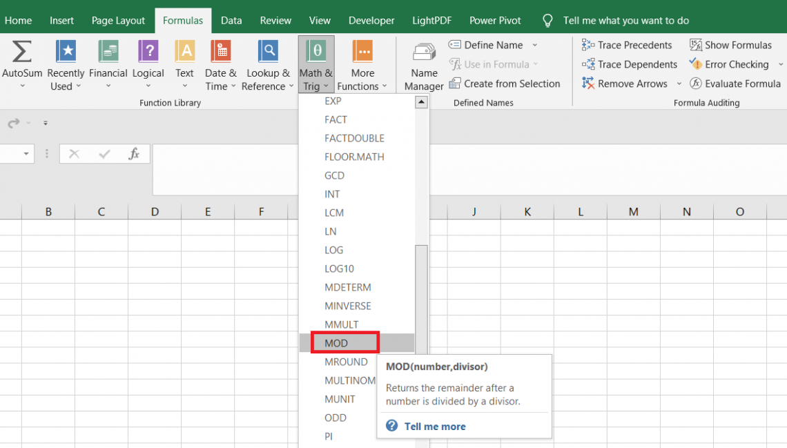
The syntax for the Mod function in Excel is:
=MOD(number,divisor)
Where,
- number - (required) the number whose remainder will be returned
- divisor - (required) the number which will be used to find the remainder
When using the function, be extremely careful with what sign the number for the divisor argument has. Generally, the result will take up the sign of the divisor, which means that if the divisor is negative, then the remainder will be negative irrespective of whether the dividend is positive or negative.
If the divisor equals zero, then Excel will return the #DIV/0! Error.
- The MOD is categorized as a Math & Trigonometric function that returns a remainder from a dividend using a divisor.
- The remainder returned is an integer value which can be positive or negative depending on the sign for the divisor.
- The function will give a #DIV/0! Error when the divisor is equal to zero.
- When negative numbers are involved, the MOD function uses a formula to calculate the remainder value. This includes using the INT function behind the scenes, which can bring wild swings in the value of the remainder from the expected number.
- The formula used is = Number-Divisor x INT (Number / Divisor). INT function returns the nearest integer value for a given number.
- The MOD function can be combined with the ROWS or COLUMN function to automatically capture even, odd, or any different numerical criteria-based cells.
- The function can also be combined with the SUM function to automatically calculate the ‘n’ numbered cells from a given range in the spreadsheet.
How to use the MOD Function in Excel?
You can already imagine what must be done to use the function correctly. You only need two numbers in a spreadsheet, reference those particular cells in the formula, and viola! You will get the remainder in the selected cell.
Suppose we have some numbers as illustrated below:
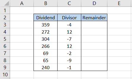
We need to find the remainder of column B numbers using column C's divisors. As you can see, some divisors are negative, while the rest are positive. Hence, the results will take the sign of the divisors in each case.
We will use the formula =MOD(B3,C3) in cell D3 and drag it down till cell D9, which gives the result:
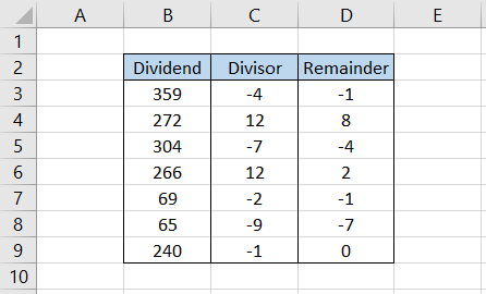
In cell B6, we have the number 266, while the divisor in cell C6 equals 12. Therefore, the number closest to 266 and divisible by 12 equals 264. Thus, when you subtract 266 and 264, you get the result as 2, the remainder obtained using the MOD function.
However, if you see the number 65 and its divisor -9, you must think that shouldn't the remainder be -2?
The closest divisible number to 65 is 63, and their difference equals 2(still, the number will take the divisor’s sign). However, that is not the case here since we get the result of -7.
The MOD function ‘sometimes’ works differently for the negative numbers. It is calculated behind the scenes using the formula:
= Number - Divisor x INT(Number / Divisor)
The INT function rounds down a number to its nearest integer value. Thus, when we divide the number and the divisor, the result equals -7.222. Rounding this figure down, we get the result as -8.
Finally, multiplying -8 by our divisor -9 gives the result of -72. When this number is subtracted from 65, the remainder equals -7. This is how we get the remainder using the function.
It can get a bit confusing, but that is how Excel works, so do not blame us here!
Getting the nth row and column using the MOD function
The function isn’t restricted to just finding the remainder for a particular number. In fact, you can even use it to get the even and odd numbered cells in the spreadsheet.
For example, you only need to highlight the odd-numbered cells in Excel.
Here, you can use the combination of MOD, ROW, and IF functions to highlight the odd-numbered cells. For example, we will use the formula =IF(MOD(ROW(A3), 2)=1, "Odd", ""), which evaluates the cell in column A and returns the result as:
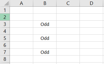
Thus, whenever the cell in column A lies in an odd-numbered row, the formula returns a customized text string as ‘Odd.’ The formula returns an empty string if the cell lies in an even-numbered row.
Similarly, you can easily highlight the even and odd numbered columns from the spreadsheet. However, the formula will change wherein we will use the MOD, COLUMN, and IF functions.
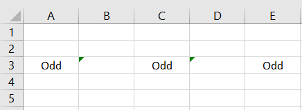
The formula becomes =IF(MOD(COLUMN(A3), 2)=1, "Odd", ""), which gives the result:
The formula is not restricted to finding the odd and even-numbered cells; you can input literally any numerical condition, and the formula will find the corresponding cells that fulfill the mentioned criteria.

SUM and MOD function
Another function that works beautifully with the MOD is the SUM function. Previously, we saw how we could find the even-numbered and odd-numbered cells.
The even-numbered cells were those whose remainder returned zero, while the odd-numbered cells were the ones whose remainder returned as one.
We can combine this idea with the SUM function to return the sum for only those numbers which are either in even or odd-numbered cells.
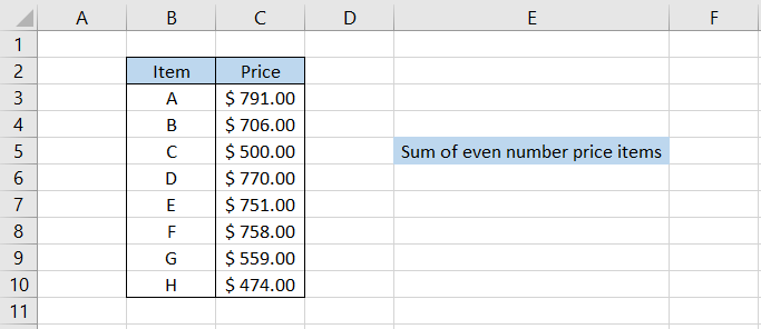
For example, suppose we have the data as illustrated below:
We will use the formula =SUM(C3:C10*(MOD(ROW(C3:C10), 2)=0)) in cell F5 and press the Ctrl + Shift + Enter key to give the result as $2708.00.
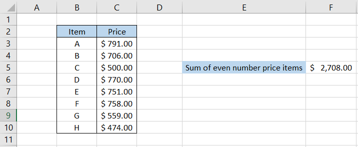
In this case, the formula adds the number in cells C4, C6, C8, and C10, i.e., $706 + $770 + $758 + $474, to give the result as $2708.
Similarly, using the SUM and MOD combination, you can calculate the sum for odd-numbered cells or any other interval.
All you need to do is add the desired condition, and the formula will automatically capture those particular cells in the final result.
Conditional Formatting & MOD function
People often overlook the versatility of the conditional formatting tool. I mean, what can it not do?

It can find a value based on predefined parameters, or you can even add unique criteria using the formulas.
Here too, we will use the MOD function to highlight particular values in a given dataset.
Suppose we have the dates as illustrated below and need to highlight all the even-numbered month dates.
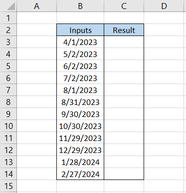
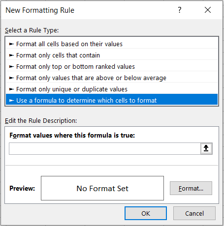
To do so, we will first highlight the range C3:C14 and then click on Conditional Formatting Tool to set up a new rule in the window as illustrated below:
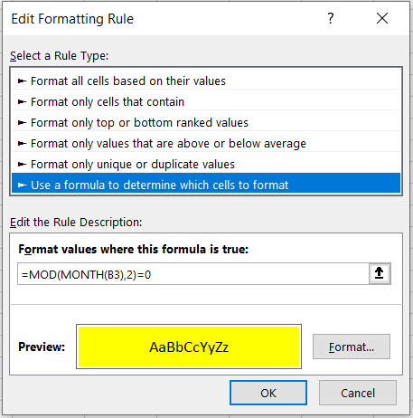
Here, we will input the formula =MOD(MONTH(B3,2)=0
This will give the result:
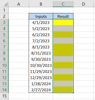
As you can see, whenever we have an even-numbered month, the formula, along with the conditional formatting tool, automatically captures the cell and highlights it for the user's convenience.
This way, you can figure out innumerable ways to use a deadly duo of MOD and conditional formatting tools!


or Want to Sign up with your social account?