MAXA Function

What is the MAXA Function?

The MAXA function in Excel finds an enormous numeric value from the range of values supplied to the function. 

You would probably argue that doesn't the MAX function perform the same task?

Well, yes, it does. It also finds the maximum value from the range of cells, but there is one big difference between both functions, i.e., the MAXA function does not ignore the logical values and the text strings.

When you input TRUE or FALSE inside the function, it will evaluate the boolean values as 1 and 0, respectively.

Similarly, inputting a text string inside the range of cells will evaluate the text string as zero.

This makes the function extremely useful when you have boolean values inside the dataset, text strings, and negative integers to determine the maximum value.

In this article, we will see the MAXA function, its syntax, and a couple of examples to understand it better.

Understanding the MAXA function

The MAXA is categorized as a Statistical function that finds the most significant numerical value from the set of numerical values, cell references with numerical values, or the range of cells, including logical values and text strings.

For example, if you have three numbers 18,36, and 21, the MAXA function will give the result as 36.

As you might be aware, the dates are represented as serial numbers; if you compare three different dates, such as 14th March 2022, 18th March 2022, and 15th March 2022, then the maximum value you would get is equal to 18th March 2022.

Talking about the significant difference, if you have three values, 0.6, 0.8, and TRUE, the function will return the maximum value as 1.

Why so?

The boolean value TRUE is equal to 1, while FALSE is equal to 0. So, when you compare the deals, the function sees those numbers as 0.6, 0.8, and 1, where it finds the last number to be the largest.

MAXA function will find the largest number, including logical values and text strings. However, it will only ignore the empty cells in the referenced range of cells.

MAXA function Formula

The syntax for the function is:

=MAXA(value1, [value2])

where,

• value1 = (required) numerical value, text string, logical value, or reference to a range of cells.
• value2 = (optional) numerical value, text string, logical value, or reference to a range of cells.

You can use up to 255 additional arguments in the function, i.e., value1, value2….value256, either directly as hardcoded values or as a referenced range of cells.

The function can be used from the library or as a worksheet formula. We will see both methods to help you decide what works best.

Method 1: From the function's library

Using the function from the library is easy, but it is not the best method if you are looking to become an Excel wizard. 

However, if you have just started the journey, understanding how the function works from the library would work wonders for you in the long term.

To use the function from the library, please follow the steps below:

1.  First, select the cell in which you intend to get the result.
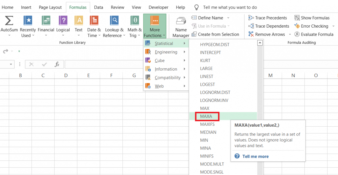
2. Click on the Formulas tab > More Functions > Statistical > select MAXA function from the drop-down, which opens the dialog box, as illustrated below:
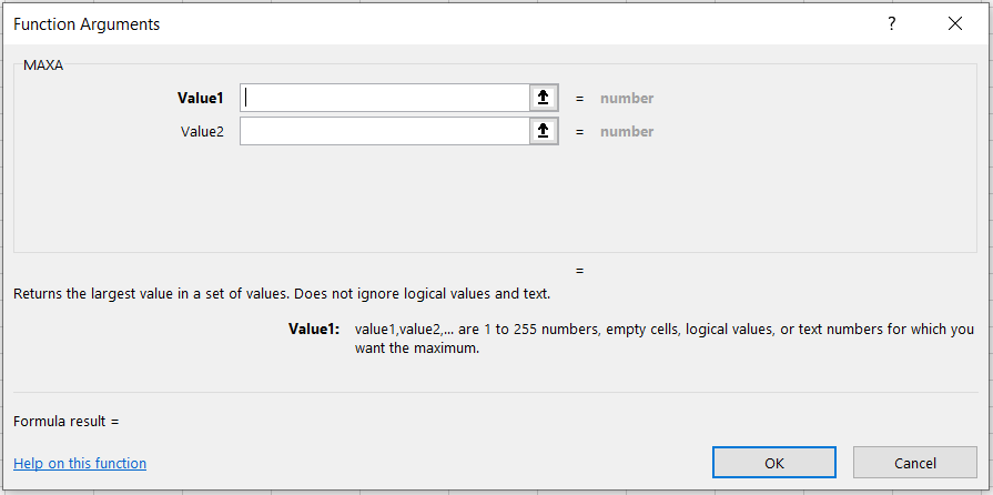
3. Here, we can directly reference the cells from the workbook for the respective values or hardcode them directly.
   We will input the three values as 10, 20, and 30 as below: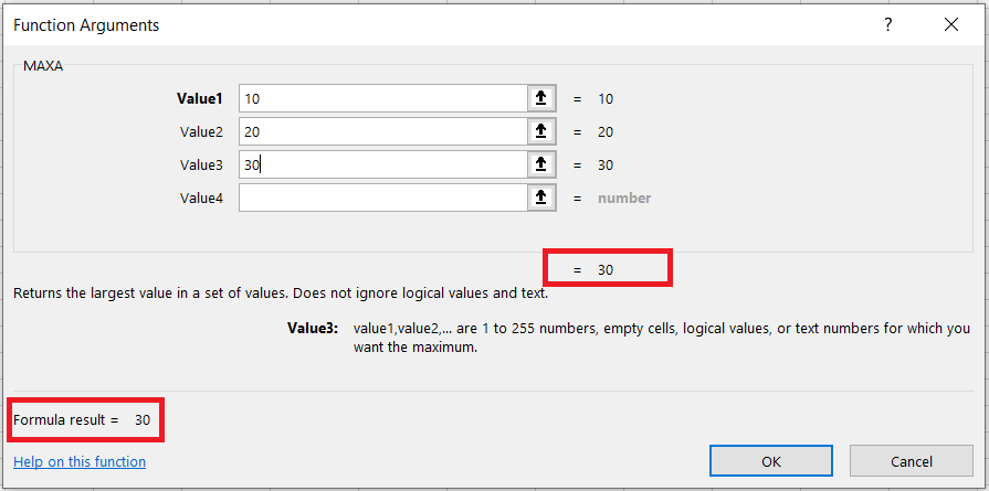
4. As you can see, we get the preview of the most significant value from the range of values we supplied in the function.
5. When you click OK, you will get the same result in the selected cell, which equals 30.

Method 2: As a worksheet formula

The easiest method and the one that will help you perform diversified analysis on a dataset in Excel.

To use the function as a worksheet formula, you must begin with an equal sign(=), type in the function name, and input the arguments inside the parentheses.

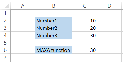
Suppose you have three numbers, as illustrated below:

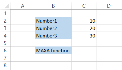
To find the maximum value, we will use the formula =MAXA(C2:C4) in cell C6, giving us 30.

In the next section, we will see examples of how the function interacts with the logical values and text strings.

How to use the MAXA Function in Excel?

We already know the function's effect on numerical values, i.e., it will find the largest value and return it to the user. But what about the logical values and text strings?

In this section, we will explore the effect of the function apart from numerical values.

Example 1: Boolean Values

A boolean value can either be TRUE or FALSE, where the former is equal to 1 while the latter is equal to 0.

Suppose you have the data as illustrated below:

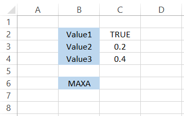
When you use the formula =MAXA(C2:C4), you get the result equal to 1, which in our dataset is Value1.

But how does that differ from the result we would get for the MAX function?

When you use the formula as =MAX(C2:C4), you will get the result as 0.4, which is the Value3.

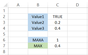
The boolean value TRUE gets ignored in the MAX function.

On the other hand, suppose you have values in Excel as below:

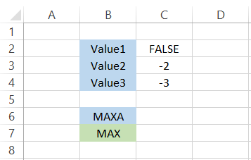
Then, by using the formula =MAXA(C2:C4) in cell C6 and =MAX(C2:C4) in cell C7, we get the result as 0 and -2, respectively.

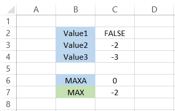
The value FALSE stored as zero gets evaluated as the maximum value for the former function, whereas, for the MAX function, it ignores the boolean value and receives the next most significant value from the dataset.

Example 2: Text Strings

Text strings are another set of values evaluated as zero in the dataset.

Let's assume that you have values in the spreadsheet as illustrated below:

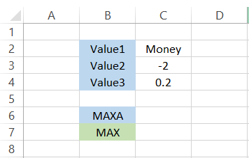
Here, we will also use the formula =MAXA(C2:C4) in cell C6 and =MAX(C2:C4) in cell C7 to get a comparative result of 0 and -2, respectively, for both functions. 

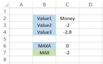
Since two of three values are negative in our data and one is a text string equalling zero, we get the maximum value as 0 in cell C6.

On the other hand, since the MAX function ignores the text strings in the results, we get the next most enormous value, which is -2 in cell C7.

Example 3: Maximum value in a general dataset

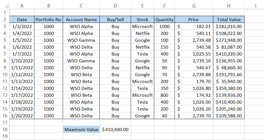
Assume we have the trade book data, as illustrated below. Next, we must find the most prominent transaction value for the last 20 days.

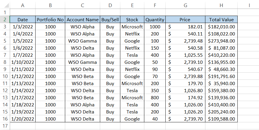
For this, you will use the formula =MAXA(H3:H16), which will run a detailed scan through column H and return the largest transaction value as $410,400. Easy peasy, right?

We forgot to mention that the MAXA function works well in collaboration with some of the logical, lookup/reference, and statistical procedures.

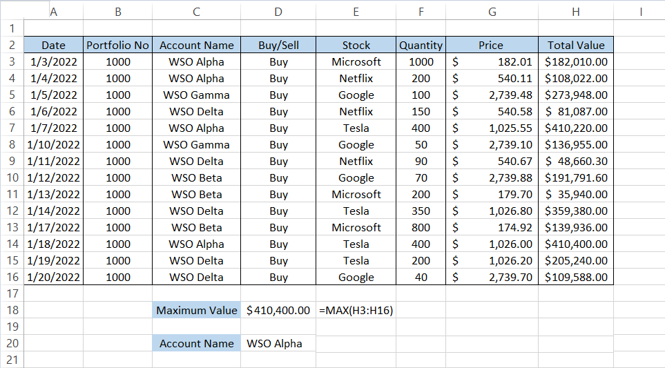
Suppose we want to return the 'Account Name' for the largest transaction value from our dataset.

The combination of INDEX-MATCH and the MAXA will give us the 'Account Name' for the most significant transaction value. 

We will use the formula =INDEX(C3:C16,MATCH(MAXA(H3:H16),H3:H16,0)), which will give us the 'Account Name' as WSO Alpha.

This way, you can use the INDEX-MATCH, VLOOKUP, or even XLOOKUP to return a value corresponding to an immense value from the dataset. 

MAXA and other functions

Some functions go well with others and help to take the data analysis one step further, and one of those versatile functions is MAXA.

This section will use the MAXA with two of the most important functions in Excel - IF statements.

a) MAXA and IF

Excel does not have any specific function that takes in a single criterion and lets you find the largest value based on the requirements.

The SUMIF function returns the sum of the numerical values that meet specific criteria, while the COUNTIF returns the count of the cells based on the condition you input.

So how do you create a function that returns the most significant value based on the range of cells meeting the given criteria?

Assume that you are a day trader and have undertaken trades as illustrated below:

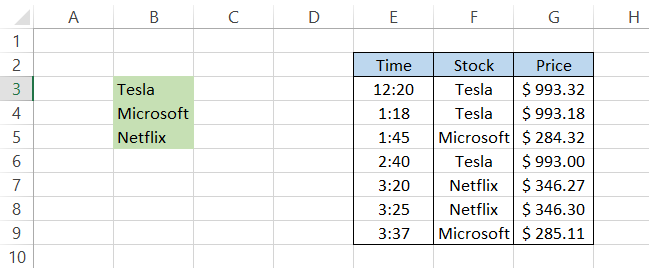
It would help if you found the maximum price paid for each stock from the recurring trades taken for the day.

To check for the maximum value, we will use the formula =MAXA(IF(B3=$F$3:$F$9,$G$3:$G$9)) in cell C3, which gives the result as $993.32.

After dragging down the formula to cell C5, we get the result:

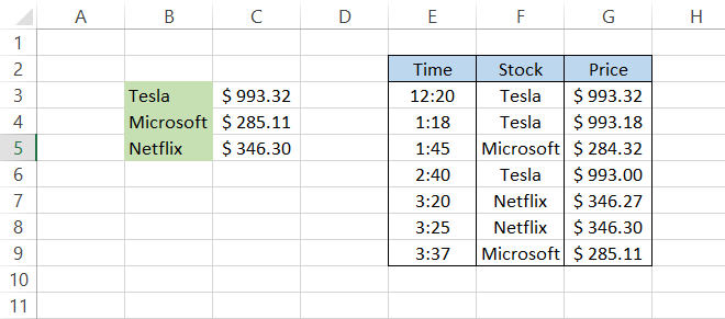
The maximum price for Tesla is $993.32, Microsoft is $285.11, and Netflix is $346.30.

b) MAXA and nested IF

Well, what about multiple conditions?

It's not like you would always be working on a single criterion. So, for example, there might be instances when you want the largest value, say, greater than 12 but less than 15.

In such a case, you can use the nested IF or multiple IF statements and the MAXA function to find the largest value.

Assume that you have trade book data, as illustrated below:

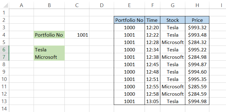
You need to find the maximum price you paid for both Tesla and Microsoft in 'Portfolio No 1001.

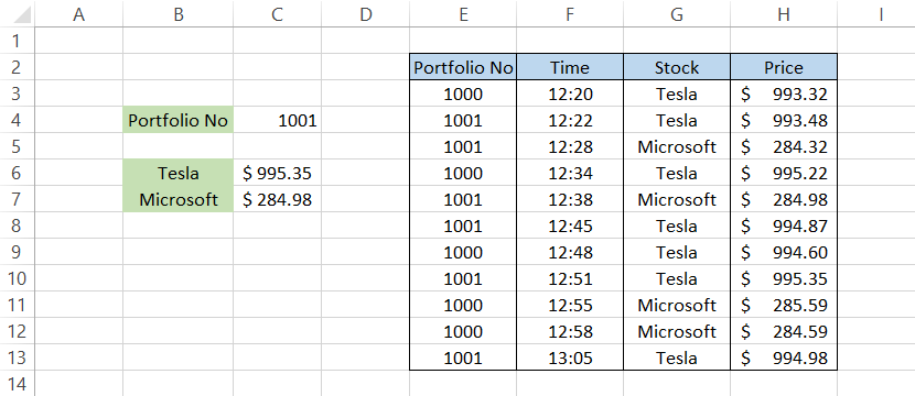
To get the result, we will use the formula =MAXA(IF(B6=$G$3:$G$13,IF($C$4=$E$3:$E$13,$H$3:$H$13))) in cell C6 to get the price for Tesla as $995.35.

Similarly, after copying the formula in cell C7, we will get the maximum price paid for Microsoft as $284.98.

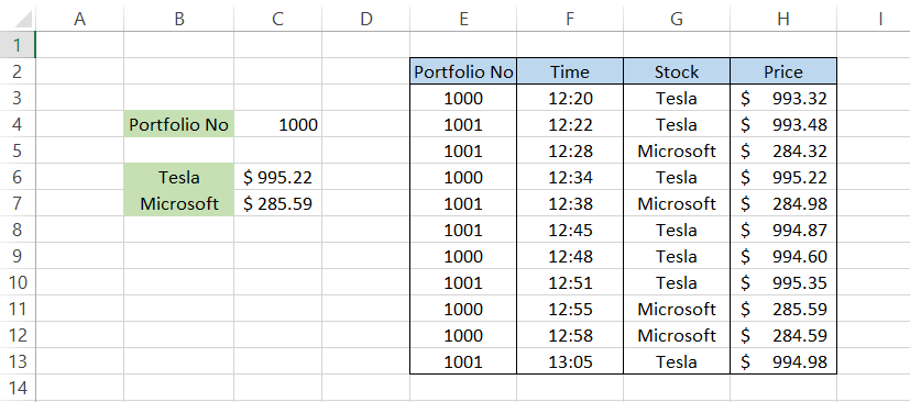
If you change the 'Portfolio No' to 1000, then the prices for both stocks will change to $995.22 and $285.59, respectively.

The only question to be answered is - how does the formula work?

1. Using the initial IF function, we evaluate and find a match for all the portfolio numbers equal to 1001 in the range E3:E13. Since this is an array formula, we get a TRUE or a FALSE if a game is found.
2. The resultant array for the first condition would be {FALSE, TRUE, TRUE, FALSE, TRUE, TRUE, FALSE, TRUE, FALSE, FALSE, TRUE}.
3. The second IF statement evaluates the range G3:G13 to find 'Tesla,' which gives the resultant array as {TRUE, TRUE, FALSE, TRUE, FALSE, TRUE, TRUE, TRUE, FALSE, FALSE, TRUE}.
4. When you combine both these arrays, we will get the resultant array as {FALSE, TRUE, FALSE, FALSE, FALSE, TRUE, FALSE, TRUE, FALSE, FALSE, TRUE}.
5. Based on the resultant array, the final four prices are $993.48, $994.87, $995.35, and $994.98.
6. Finally, the MAXA function works magic to give the most significant value from this resultant array, which equals $995.35.

The conditional arrays mentioned above are for 'Tesla' and would change for condition 'Microsoft.'

Researched and Authored by Akash Bagul | Linkedin

Reviewed and edited by Parul Gupta | LinkedIn

Free Resources

To continue learning and advancing your career, check out these additional helpful WSO resources:

• HOUR Function
• HYPERLINK Function
• PEARSON Function
• PI Function
• SEARCH Function