PROB Function

What is the PROB Function?

A prob function is a mathematical function describing the likelihood of distinct outcomes in a random event.

In the prob theory, a numeral between 0 and 1 exemplifies an event’s likelihood. Here, zero signifies the occasion will not occur, and one suggests the occasion will arise.

It allocates a probability to each possible random event’s output. The sum of all the probabilities of the probable outcome equals 1.

History of the probability function: Several mathematicians and philosophers have studied the concept of probability over the years. However, many scholars developed the "modern mathematical theory of probability" in the 17th and 18th centuries. These include

1. Blaise Pascal: A French mathematician, physicist, and philosopher 
He is credited with laying the foundations of the 'modern theory of probability.' His famous works comprise the concept of expected value and the principle of least expectation.

2. Pierre-Simon Laplace: A French mathematician and astronomer 
Laplace devised probability theory at the end of the 18th and the beginning of the 19th century.
He is known for his work on the probability of events occurring in repeated trials and his thoughts on the normal distribution, describing the probability of continuous random variables.

3. Jakob Bernoulli: A Swiss mathematician 
He is famous for his work on the probability of events occurring in a row and mathematical expectation, which describes the average value of a random variable over many trials.

Formula for a probability function

The formula for the function assigns a probability to each random event's probable output. The general form of the likelihood (probability) function is:

P(X) = prob of event X occurring.

Where, 

• X is a random variable depicting the possible outcomes of the event.

To understand the concepts of probability and chance, the most classic example given by scholars is a 'coin flip.' The prob function for this event would assign a probability of 0.5 (or 50%) to the outcome "heads" and "tails" since each result has an equal chance of occurrence.

If the random variable X represents the result of the coin flip, the likelihood function for this event would be written as P(X).

To illustrate condition 2, let's assume the likelihood function for a six-sided dice roll. It is represented as:

• P(1) = 1/6
• P(2) = 1/6
• P(3) = 1/6
• P(4) = 1/6
• P(5) = 1/6
• P(6) = 1/6

Then the likelihood of each output (i.e., rolling a 1, 2, 3, 4, 5, or 6 on dice) is 1/6, and the summation of the probabilities of all probable outcomes is P(1) + P(2) + P(3) + P(4) + P(5) + P(6), i.e., 1/6 + 1/6 + 1/6 + 1/6 + 1/6 + 1/6 = 1.

Types of Probability Functions and their formulas

Various prob functions describe the likelihood of different outcomes in a random event.

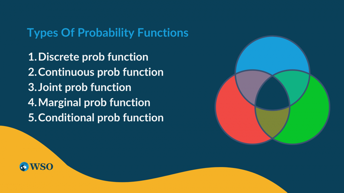
Some of the most common types of probability functions include:

1. Discrete prob function

This function describes the likelihood of a discrete random variable, a random variable that can take on only a finite or countably infinite different value.

The formula can be seen as follows:

P(X = x) = prob of X taking on the value x

Where, 

• X is a discrete random variable, and x is a specific value that X can take.

Illustration: The number of heads that come up in a series of coin flips is a discrete random variable. The probability function for this event would be:

P(X = "heads") = 0.5

P(X = "tails") = 0.5

Where X is the random variable representing the outcome of the coin flip.

2. Continuous prob function

This function describes the likelihood of a continuous random variable, which is a random variable that can take on any value within a specific range.

The formula can be seen as follows:

f(x) = probability density function

P(a <= X <= b) = integral of f(x) from a to b

Where 

• X is a continuous random variable
• f(x) is the probability density function (PDF) for X
• a and b are specific values within the range of possible values for X.

Illustration: The height of a randomly selected person represents a continuous random variable. The probability function for this event might be described by a normal distribution with a mean of 70 inches and a standard deviation of 3 inches:

f(x) = (1 / (3 * sqrt(2 * pi))) * exp(-((x - 70)^2) / (2 * 3^2))

Where x is the person's height in inches and f(x) is the PDF for the person's height.

3. Joint prob function

The JPF function describes the likelihood of two or more random variables occurring jointly. The formula can be seen as follows:

P(X = x, Y = y) = prob of X taking on the value x and Y taking on the value y

where 

• X and Y are random variables
• x and y are distinct values taken by these random variables, respectively.

Illustration: Consider the JPF for heads and tails appearing in a sequel of tosses representing the likelihood of various combinations of heads (H) and tails (T). As a result, the combinations seen are HH, HT, TH, and TT.

The JPF for this event would be:

P(X = "H", Y = "T") = 0.25

P(X = "H", Y = "H") = 0.25

P(X = "T", Y = "H") = 0.25

P(X = "T", Y = "T") = 0.25

Where X and Y are the random variables representing the output of the first and second coin toss, respectively.

4. Marginal prob function 

This function defines the likelihood of a single random variable occurring, irrespective of the value of other random variables.

The formula can be seen as follows:

P(X = x) = sum of P(X = x, Y = y) over all possible values of y

where 

• X and Y are random variables
• x and y are specific values these random variables can take.

Illustration: Elaborating on the example above, let's consider the MPF for the number of heads appearing in a sequence of coin tosses. It expresses the likelihood of heads occurring, irrespective of how many tails appear.

The MPF for the number of heads appearing in the two flips would be:

P(X = 0) = 0.25

P(X = 1) = 0.5

P(X = 2) = 0.25

Where X represents the number of heads that come up in the two tosses.

5. Conditional prob function 

The function describes the likelihood of a random variable occurring given that some other event has happened. The formula can be seen as follows:

P(X = x | Y = y) = P(X = x, Y = y) / P(Y = y)

where 

• X and Y are random variables 
• x and y are specific values X and Y can take, respectively.

Illustration: To understand the CPF for the number of heads appearing in a sequel of tosses, assume that the total number of heads and tails is even. It would denote the likelihood of heads occurring, with the condition that the entire heads and tails happening is even.

The CPF would be:

P(X = 0 | X + Y = 0) = 1.0

P(X = 1 | X + Y = 2) = 0.5

P(X = 2 | X + Y = 2) = 0.5

Where X and Y denote the number of times heads and tails appear in the two tosses, respectively.

Advantages and Disadvantages of Using Probability Functions

The primary benefits of utilizing likelihood capabilities to depict the probability of different results on a rare occasion incorporate the accompanying:

1. They give a numerical structure to understanding and foreseeing the results of rare occasions. Relegating a likelihood to every possible outcome permits us to measure the vulnerability related to an event and make forecasts about the probability of various effects happening.
2. They permit us to break down the connections between various irregular factors and to comprehend how they impact each other.
3. They help break down and think about various situations or occasions. By contrasting the likelihood elements of multiple occasions, we can figure out which event is bound to happen or which significantly affects the general likelihood of a result.
4. They help dynamic under vulnerability. For instance, by utilizing likelihood capabilities to comprehend the probability of mixed results, we can settle on informed conclusions about designating assets or answering various situations.
5. They help in demonstrating and breaking down certifiable peculiarities. We can acquire experiences into complex frameworks and anticipate how they might act.

The primary weaknesses are:

1. Likelihood capabilities depend on suppositions about the hidden cycles that create the results of a rare occasion. If these suspicions are wrong or fragmented, the ability may not precisely mirror the genuine probability of outcomes.
2. The precision of the prob capabilities relies upon the information used to gauge them. For instance, if the data used to gauge a likelihood capability is restricted or one-sided, the subsequent capacity may not precisely mirror the genuine probability of results.
3. They can be hard to decipher and impart to others, particularly assuming they depend on complex models or include irregular factors.
4. They may not represent all variables impacting the result of a rare occasion. Now and again, extra factors or wellsprings of vulnerability can influence the precision of expectations made utilizing the capability.
5. They might be delicate to little changes in the information or assessment suspicions. This can make it hard to precisely foresee the probability of various results happening over the long run.

PROB functions in Excel

Excel is a spreadsheet software program that performs various statistical and mathematical calculations, including probability functions.

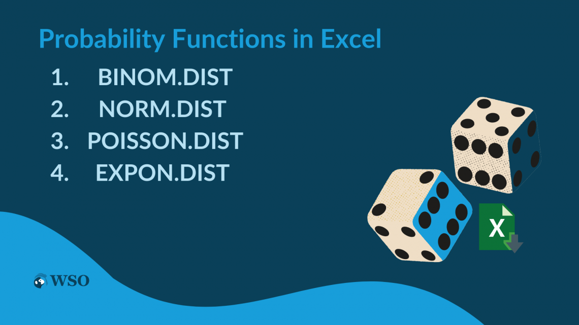
Some of the expected probability functions available in Excel include:

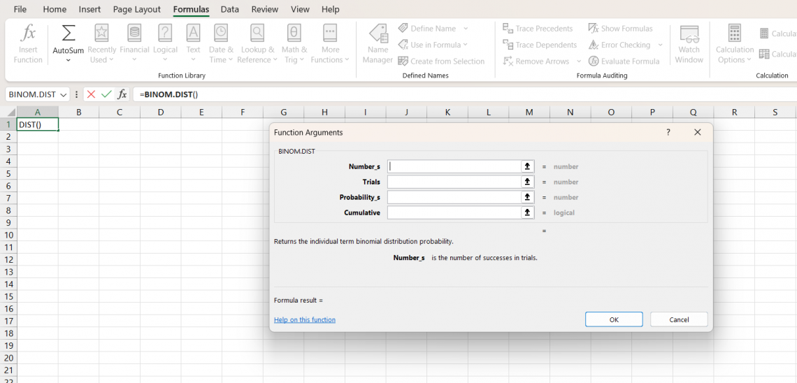
1. BINOM.DIST

This function calculates the probability of a specific number of successes in a series of Bernoulli trials, where each practice has a fixed probability of success. The syntax of the BINOM.DIST function is as follows:

BINOM.DIST(number_s, trials, probability_s, cumulative)

where 

• number_s is the number of successes in the trials
• trials represent the total number of trials
• probability_s is the probability of success for each trial 
• cumulative is a logical value that specifies whether to return the cumulative probability (TRUE) or the probability mass function (FALSE).

For example,

=BINOM.DIST(3, 5, 0.5, TRUE)

This formula would return the probability of getting exactly 3 heads in 5 coin flips with a probability of 0.5 (or 50%) for each flip coming up heads. The argument is set to TRUE, so the function will return the cumulative probability of getting ≤ 3 heads in the 5 flips.

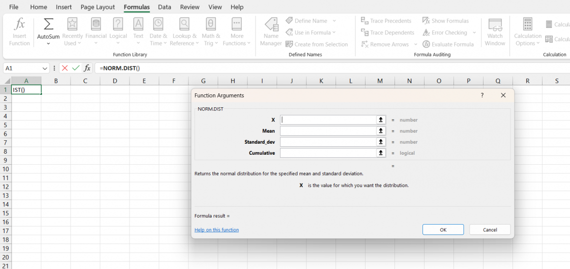
2. NORM.DIST 

This function computes a normal distribution's prob density or cumulative distribution function. The syntax or the sentence structure of the procedure is as follows:

NORM.DIST(x, mean, standard_dev, cumulative)

Where

• x is the value for which you want to estimate the likelihood, 
• mean is the expected average value of the normal distribution, 
• standard_dev is the standard deviation of the normal distribution
• cumulative is a 'logical value' specifying whether to return the cumulative likelihood (i.e., TRUE) or the probability density function (i.e., FALSE).

For example,

=NORM.DIST(70, 75, 5, TRUE)

The formula would return the cumulative prob of a value being ≤ 70 in a normal distribution with a mean and standard deviation of 75 and 5, respectively. Therefore, the argument is set to TRUE so that the function yields the cumulative prob of a value ≤ 70.

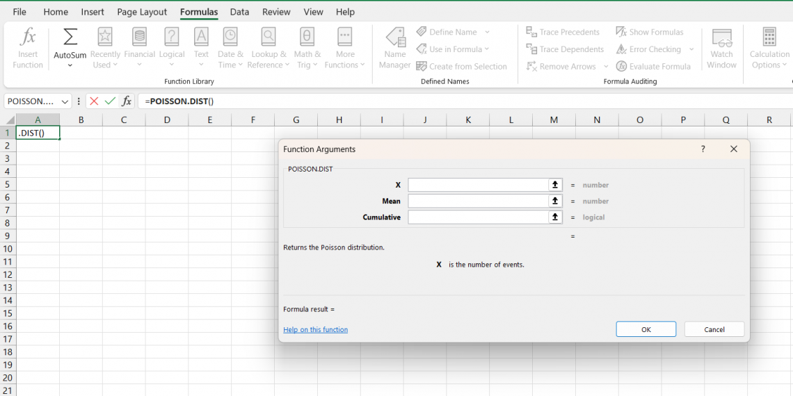
3. POISSON.DIST

This function computes the likelihood of a particular number of occasions happening in a predetermined period or space, given a steady pace of events. The syntax of the function is as follows:

POISSON.DIST(x, mean, cumulative)

where 

• x is the number of events, 
• mean is the expected number of events, 
• cumulative is a logical value that specifies whether to return the cumulative prob (TRUE) or the probability mass function (FALSE).

For example,

=POISSON.DIST(3, 5, TRUE)

The formula above gives the cumulative prob of ≤ 3 events happening in an interval given the mean value 5. The argument is set to TRUE so that the POISSON.DIST returns the cumulative prob of ≤ 3 events.

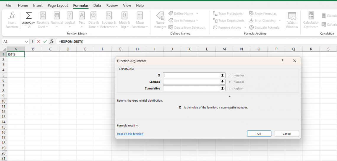
4. EXPON.DIST 

This function calculates the exponential distribution's probability density or cumulative distribution function. The syntax of the EXPON.DIST function is as follows:

EXPON.DIST(x, lambda, cumulative)

where

• x is the value for which you want to calculate the probability, 
• lambda is the rate parameter of the exponential distribution
• cumulative is a logical value specifying whether to return the cumulative probability (TRUE) or the probability density function (FALSE).

For example,

=EXPON.DIST(1, 2, TRUE)

This formula would return the cumulative probability of a value being ≤ 1 in an exponential distribution with a rate parameter of 2. The argument is set to TRUE so that the function will return the cumulative probability of a value being ≤ 1.

To use probability functions in Excel, follow these steps:

1. To use probability functions in Excel, follow these steps:
2. Open the Excel spreadsheet containing the data you want to analyze.
3. Next, select the cell where you need to enter the likelihood capability.
4. Type the capability name and opening bracket.
5. Enter the essential information contentions for the capability. Type an end enclosure and press Enter to finish the ability.
6. The capability will return the likelihood of the predetermined occasion, given your input contentions.

Researched and authored by Parul Gupta | LinkedIn

Reviewed & Edited by Ankit Sinha | LinkedIn

Free Resources

To continue learning and advancing your career, check out these additional helpful WSO resources:

• Alphabetize in Excel
• Data Validation in Excel
• Excel Drop Down List
• Excel Shortcuts
• VLOOKUP