RANK Function

What Is RANK Function?

The RANK is categorized as a Statistical function that assigns a rank to a range of supplied values and determines the position of each value within the rank.

However, when you look for the function in the library, you will find it under the Compatibility section for backward compatibility.

A function in the compatibility section means that a newer version has replaced it, but the older version is still kept so that old and new Excel files can run the function seamlessly.

However, it is still advisable to use the newer function RANK.EQ and RANK.AVG since the former function might not be available for use in the future.

Suppose that you have three numbers 10, 20, and 30. When you use the function, it will rank them in ascending or descending order, based on your preference, and return the result in the corresponding range of cells.

The syntax for the function is:

=RANK(number, ref, [order])

where,

• number: (required) the value or number which will be ranked.
• ref: (required) the list of values or the reference to the range of values against which the number argument will be compared for ranking.
• order: (optional) defines in what order to rank the given data, i.e., ascending or descending. Zero if the values are arranged in descending order, and one of the values is in ascending order.

One of those tools developed in computers is Microsoft Excel which enables the user to organize and manipulate the data and crunch numbers for the available dataset.

Microsoft Excel has a subset of several data calculation, organizing, and manipulation tools, one of which is the RANK function.

How to use the RANK function

There are two different ways you can use the function in Excel - from the function's library or as a worksheet formula. The latter method is the most preferred method of using functions by most Financial Analysts and Investment bankers.

In this section, we will explore both methods as each has its pros and cons.

a) Method #1: From the functions library

The advantage of using a library function is you better understand how the process works. However, if you are a beginner who has just started the journey to becoming an Excel wizard, we recommend you check out all the different functions in the library.

To use the function from the library, please follow the steps below:

1. Select the cell in which you intend to return the result.
2. Click on Formulas > More Functions > Compatibility and select the RANK function from the drop-down menu.
3. This will open up the dialog box, as illustrated below:
4. Here, we can directly reference the cells in the dialog box or hardcode the values. Another thing that we see is that the dialog box perfectly explains everything regarding the function, from the arguments to what it does as well as what the result is.
   We will input the arguments in the dialog box as below:
5. Based on our inputs, Josh's test scores of 75 are ranked in the second position. Press Ok and drag the result to cell D5, and you will get the rank for other test scores.
6. The drawback of the method is that it can be time-consuming and a bit rigid to use. What if you want to use multiple functions together?

This brings us to the second method, which uses the function as a worksheet formula.

b) Method #2: As a worksheet formula

Using the function as a worksheet formula is no rocket science. Even the very beginner can at least use the SUM function as a formula with zero guidance.

We begin with the equal sign in the selected cell, type in the function name, and input the arguments inside the parentheses.

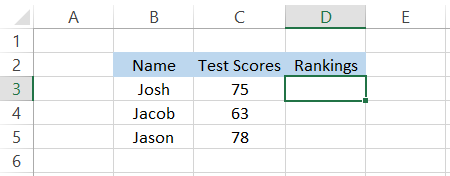
Let's say that you have test scores as illustrated below:

In cell D3, we will use the formula =RANK(C3,$C$3:$C$5,0) and drag it down to cell C5 using Ctrl + D, which gives us the ranking for the test scores as:

Based on the result, we can interpret that Jason scored the highest on his test, followed by Josh, standing at second rank, and Jacob at the third rank.

An important thing to remember while referencing the ref argument is to fix them using the dollar sign($), or else you might get the wrong results in Excel.

Example of the RANK function

This section will show a few examples to help you understand the function better. By now, this might be clear to you that the part primarily works on numbers or any data type derived from numbers such as date and time.

However, the function would not work on text values and would instead return a #VALUE! Error.

a) Example #1

Suppose you are a swing trader and make a series of trades for your portfolio. After a few weeks, you close all the work. As a final step, you must evaluate the stocks with the highest and lowest profits.

Suppose that you have the data as illustrated below:

To rank the stocks based on their profit, we will use the formula =RANK(J3,$J$3:$J$7,0) in cell K3 and drag it down to K7, which gives us the result:

Based on the profits, you will see that Apple Inc is ranked first while Meta Inc is rated last in the series. Since we used the order argument as descending, we get the highest to lowest profit ranking.

Suppose we need the ranking for lowest to highest profit. In that case, we will tweak the formula to =RANK(J3,$J$3:$J$7,1), i.e., change the order argument to ascending, which gives the updated rankings, as illustrated below:

Based on ascending order, we see that Meta Inc has the lowest profit from the lot while Apple Inc has the highest.

Thus, the function makes ranking numbers easier in Excel.

b) Example #2

We know that date is stored as a serial number while time is stored as a decimal number in Excel. Based on this information, we can assign ranks to those date and time values and categorize what date/time comes first and what comes last.

Suppose you work at Amazon in the order fulfillment department. It would help if you prioritized the orders based on the time or date they were ordered.

The data looks, as illustrated below:

 Here, we will use the formula =RANK(D3,$D$3:$D$12,1), which gives us the result:

As per the order time in the database, the first order that needs to go out is for Vickie Tate(no, not related to Andrew Tate in any way) at 12:35:40 AM.

Remember that we have assigned the ranks in ascending order, and hence the first rank would be assigned to the time that is the earliest in the 24-hour clock.

Similarly, if you had different order dates in the dataset, we would use a similar formula =RANK(D3,$D$3:$D$12,1), which gives the result:

One thing you would notice is that if the date value is similar, the rank assigned to both is also the same. So, for example, Colin Parsons and Gustavo Vaughn have the same order date, and hence they have the same rank.

When two values have the same rank, we observe that the next level is skipped, which in this case is 4. No date in our dataset is assigned the rank 4.

What is RANK.EQ

The RANK.EQ is categorized as a Statistical function that assigns a rank to a range of supplied values and determines the position of each value within the class.

Excel introduced two newer versions for the RANK function, amongst which RANK.EQ is the closest exact match for the function.

You might wonder, if both of them perform the same task, why was there even a need to introduce a newer version?

The answer is simple - to offer Excel users more flexibility in data analysis and number crunching. You can also imagine it in a way where the primary function is branched into two different tasks while there is still much more potential to add more parts.

The syntax for the function is:

=RANK.EQ(number, ref, [order])

where,

number - (required) the value or number which will be ranked.

Ref - (required) the list of values or the reference to the range of values against which the number argument will be compared for ranking.

order - (optional) defines in what order to rank the data, i.e., ascending or descending.

Suppose that you have the data as illustrated below:

We will use the formula =RANK.EQ(C3,$C$3:$C$5,0) in cell D3 and drag it down to cell D5, which gives the result:

We did say that the function comes closest to the 'former' RANK function. To compare both of their results, we will use the formula =RANK(C3,$C$3:$C$5,0) in cell E3 and drag it down to cell E5, which gives us the same results in both columns.

Even though this article is based on the previous version RANK function, we still advise you to use RANK.EQ from now on to assign positions to the numerical values.

Note: An important thing to remember is that if the function finds two same numerical values, it will assign the same rank. For example, if two test scores of 75 are in the dataset, they would be given level 2.

However, the number next in line would be assigned rank 4 and not 3 as the function skips a class when it finds duplicate numerical values.

what is RANK.AVG

The one significant difference that the RANK.AVG function portrays that it will assign the mean value as a rank if there are two or more similar values in the dataset.

The RANK.AVG is categorized as a statistical function that 'also' returns the rank for the value. However, if one or more similar values exist, then Excel assigns an average level to those values.

The syntax for the function is:

=RANK.AVG(number, ref, [order])

where,

• number - (required) the value or number which will be ranked
• ref - (required) the list of values or the reference to the range of values against which the number argument will be compared for the ranking.
• order - (optional) defines in what order to rank the data, i.e., ascending or descending

Let's see an example to understand what average rank the function returns for the same numerical values. Suppose that you have the data as illustrated below:

Notice that we have two people with an equal test score of 64. We will use the formula =RANK.AVG(C3,$C$3:$C$8,0) in cell D3 and drag it down to cell D8, which gives the result:

On the contrary, when you use the =RANK.EQ(C3,$C$3:$C$8,0), you get the result as:

When the function finds a similar numerical value, it usually skips a rank which in both cases is rank 4.

Practical Example of RANK Function

You thought this was the end of the article, didn't ya? Well, bear with us for a few more examples that could probably help you a lot in your professional life.

We saw that each of those three functions skips a rank and simultaneously assigns the same level when you reference the same numerical value.

But what if you wanted unique ranks for each of the values in the dataset?

In this case, we will combine COUNTIF and the RANK function.

Suppose you have the data, as illustrated below:

To find the unique ranks, we will use the formula =RANK(C3,$C$3:$C$12,0)+COUNTIF($C$3:C3, C3)-1 in cell D3 and drag it down to cell D12, which gives the result:

As you can see, whenever the formula finds a duplicate value(test score), the rank assigned is still unique. But what is the criterion for unique ranking?

The unique rankings are assigned based on what value Excel finds first in the referenced range. 

For example, Jody Mendoza is the first student who scored 64 on his history test and is assigned a unique rank of 5, followed by Ruth Thompson, who is given a level of 6.

If we had used the traditional RANK function using the formula =RANK(C3,$C$3:$C$12,0), we would get the result:

Thus, you can use either the traditional function to assign positions to numerical values or give them unique ranks based on the above formula in Excel. 

Researched and authored by Akash Bagul | LinkedIn

Reviewed and edited by Parul Gupta | LinkedIn

Free Resources

To continue learning and advancing your career, check out these additional helpful WSO resources:

• CODE Function
• HOUR Function
• PI Function
• YEAR Function
• YIELD Function