REPT Function

What is the REPT function?

REPT is categorized as a Text function that repeats text 'n' many times. The REPT function in Excel will repeat a character or a text string ‘n’ a number of times.

There would be a limited number of scenarios where you might need to repeat a particular character or a text string in a dataset.

Rather than editing the cell by pressing F2 and then typing the desired string repeatedly or even using the Ctrl + C / Ctrl + P combo, the REPT function provides a more reliable source to input characters or input text strings that keep repeating up to a certain extent.

However, there is a limit to the number of characters that can be repeated using the function, which equals 32,767. If you go beyond this number, the function returns the #VALUE! Error.

We know that Excel allows us to input characters that accommodate multiple cells in the spreadsheet. But have you heard of charts inside a single cell?

You heard it right. The function allows us to create in-cell charts and find the last text entry in the column, similar to finding the last cell in a VBA code.

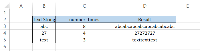
The function can fill a cell with an 'n' number of instances of a text string limited to 32,767 characters. For example, if you have the text string as 'abc' and use the function to repeat the text 5 times, then the result you would get would be equal to 'abcabcabcabcabc.'

Similarly, if you had a numerical value equal to 27 and needed to repeat it four times then using the function, you would get the result 27272727. Generally, when we say that the numerical value or text string would repeat 'four times, we assume the repetitions are apart from the original value.

However, that is not the case. When you use the function, the original value is included in the number of instances as the final REPT value, i.e., one actual + three repeated values give us the result as four repeated instances.

The syntax for the function is:

=REPT(text, number_times)

where,

• text = (required) the text string that we intend to repeat
• number_times = (required) number of times the text string will be repeated

An important thing to remember is that the function can only store and return 32,767 characters as our result. If the number of characters in the text string returned using the REPT function exceeds that number, we will get the #VALUE! Error.

 How to use the REPT function?

To use the function, head over to the cell where you expect the result. Begin with an equal sign, type in the function name, and input the arguments inside the function.

You can either hardcode both arguments or reference the cell in the formula.

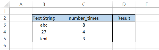
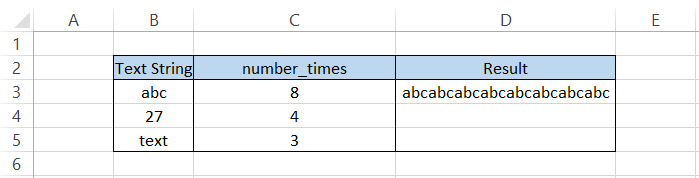
The formula in cell D3 would be =REPT(B3, C3) which would give you the result as 'abcabcabcabcabcabcabcabc.'

The alternate formula with hardcoded values would be =REPT("abc," 8), which would give the same result as:

Similarly, by copying the formula down in cells D4 and D5, we get the result:

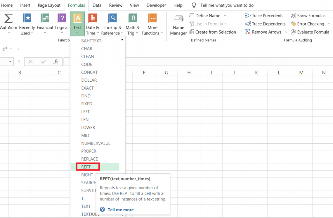
You can use the alternate method via the function's library, which you will find under the Formulas tab.

First, select the cell in which you expect the result, click on Formulas tab > Text, and then choose REPT from the drop-down menu to open the dialog box as illustrated below:

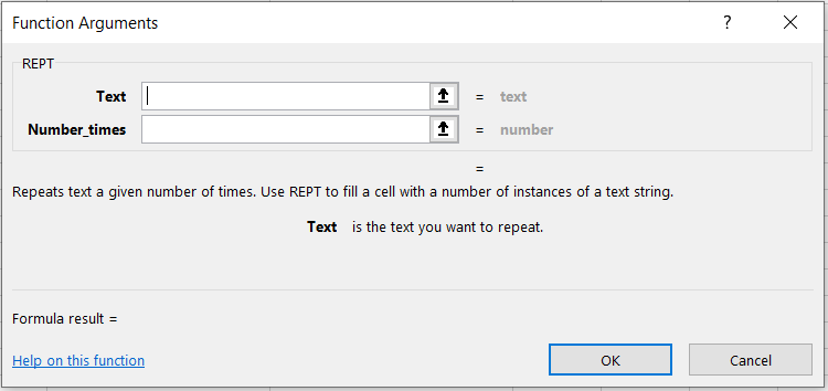
Either hardcode the arguments or directly input the cell references. Here, we input the text as 'abc' and number_times as 8 like:

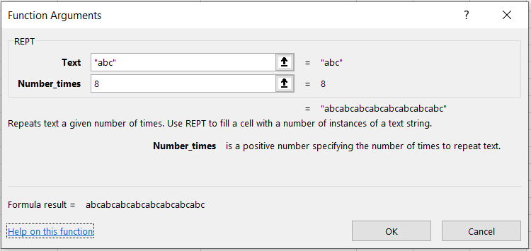
When you click on OK, you get the same result. However, most Excel users prefer to use the function as a worksheet formula since it is a much easier and time-saving method.

Example for the REPT function

We guess it's clear that the function will repeat a given text string 'n' several times. So we don't believe that we need to see those simple examples anymore.

We will see how you can use the function to get the exact length of numerical values. Unfortunately, it isn't easy to compare numerical values when they are of different sizes.

For example, consider two revenues $1,121,231 and $1,281,923,981. You might probably make mistakes while making arithmetic calculations such as addition, subtraction, multiplication, etc.

The function also allows us to create in-cell graphs using specific characters. You would ask," Why is there a need to develop in-cell diagrams when we could create charts directly?"

An in-cell graph takes less space as compared to traditional charts or graphs. Besides, if there is just a single value for which you intend to plot a graph, then in-cell diagrams work.

Let's see some complex examples of where the REPT function would be used to help make life far more accessible.

Example #1: Making numerical values of the same length

It isn't easy to compare numbers with variable lengths, especially if you are working on financial models or other financial information.

The numbers can be easily misinterpreted if they are not the same length, even for simple arithmetic calculations such as addition and subtraction.

Suppose the data looks as illustrated below:

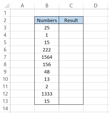
To make the numbers of equal length, we will use the formula =REPT("0",4-LEN(B3))&B3 in cell C3 and drag it down till cell C13 which gives the result:

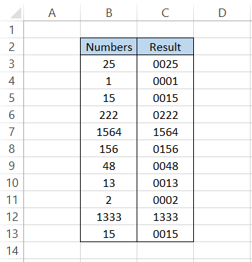
The formula adds leading zeros to the numbers in the dataset. As you can see in the procedure, we input the number 4 and then subtract the length of the text string to get the number_times argument for the formula.

But wait, that's a hardcoded value. That would mean amendments to the formula if we have numbers more significant than length four. Should we directly input a more significant number, say 10 instead of 4, in the formula? 

No need for that. We will nest the MAX function such that the updated formula becomes  =REPT("0",LEN(MAX($B$3:$B$13))-LEN(B3))&B3 in column C. Now, change the number in cell B4 to 1354654. The result that you would get is:

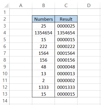
As you can see, the function identifies the most significant number, 1354654, takes its length, and then subtracts the distance from each number in column B to add the leading zeros in the numbers.

Example #2: Creating in-cell charts

Suppose you decide to illustrate the student's English test scores using the in-cell charts.

The data looks as illustrated below:

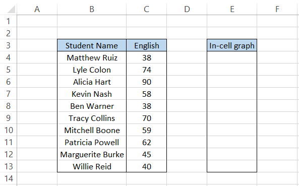
We know that the test score's upper and lower limits would be 100 and zero, respectively.

To create our in-cell chart, we will first select a symbol or a character that will act as our marker for the test scores.

For this, click on the Insert tab > Symbols > select any font(preferably Arial Black and then insert the complete block symbol in cell D1

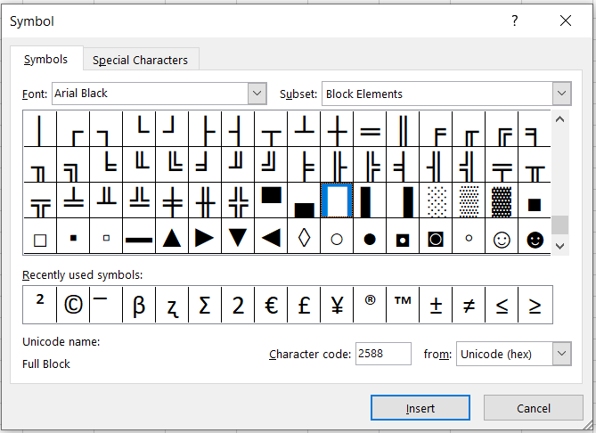
The second criterion you need to keep in mind is selecting monospaced fonts, i.e., they have equal spaces between the characters. A great example of monospaced font is the Courier New font.

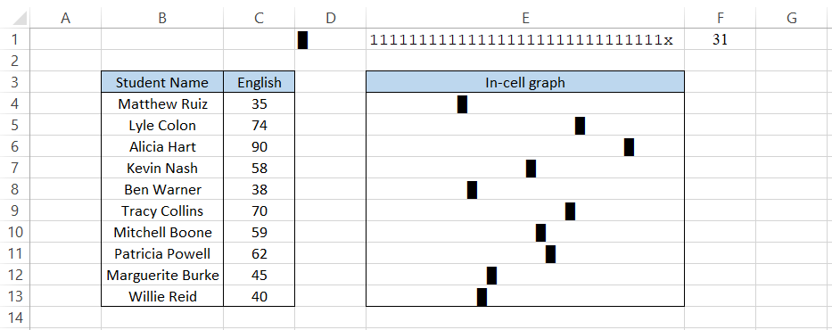
We will input the =REPT("1",30)& "x" in cell E1, which would give us the range of the in-cell chart. Then, in cell F1, we will calculate the length of the text string returned in E1, which will be next used in another formula.

So far, the spreadsheet looks as illustrated below:

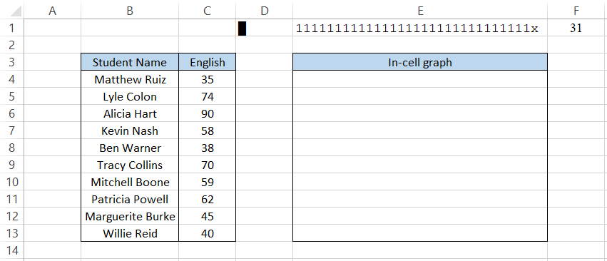
Finally, we will use the formula =REPT("",MAX(0,(C4-0)/(100-0)*$F$1-1))&$D$1 in cell E4 and drag it down to cell E13 which gives the result:

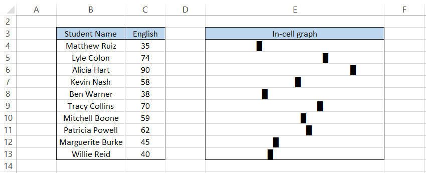
The left end of the in-cell graph has the assumed value of zero, while the right end has a discount equal to 100.

Since the graph is plotted, you can choose to hide the first column directly, which gives us the result:

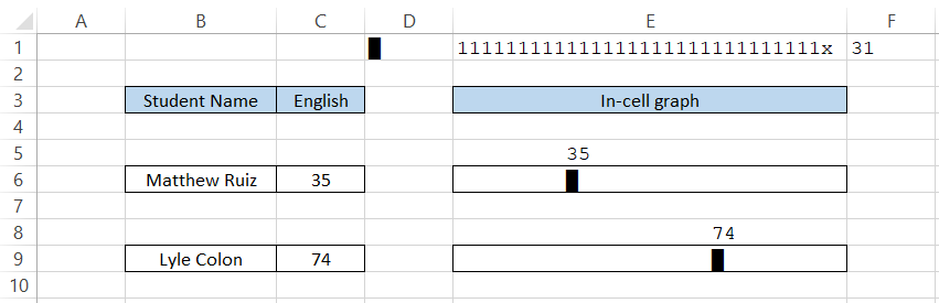
Another formula would display the test scores above the in-cell graphs but might make the chart messy.

Nevertheless, if you wish to use it as well, you can use the formula =REPT("", MAX(0,(C6-0)/(100-0)*$F$1-1))&$C$6 in the cell above the in-cell graph.

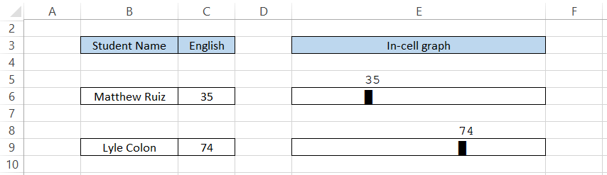
For example, cell E5 is placed above cell E6, which contains the in-cell graph. We have used the formula in the E5 cell, which gives us the English test score above the in-cell chart.

How does the formula work?

• Firstly, we use the space character( ) as the text string that will be repeated for 'n' several times.

• For the number_times argument, the formula has two choices - either select zero if it is the maximum value or selects the result from the arithmetic formula (Test Score - Minimum Value) / (Maximum Value - Minimum Value) * Length of a text string in cell E1-1)

• We know that the minimum value for the test score is 0 while the maximum is 100. If you are creating an in-cell graph, let's say for stocks, then you can either hardcode the minimum and maximum price or input them in separate cells to reference in the formula.

• The result of (Test Score - Minimum Value) / (Maximum Value - Minimum Value) or (35-0)/(100-0) is equal to 0.35, which then gets multiplied by the string in cell E1, which gives the result of 9.85.

• Remember that we had a total of 31 characters in cell E1, so 9.85 means the graph has covered 9 characters completely and 0.85 of the final character.

• If the test score was, let's say, 98, then the marker would be at the 30th character. We subtract one from the formula to have a buffer for the tag in the graph.

• We know that's quite a lot of information and somewhat confusing, but the bottom line is that the formula helps to divide the test score into equal intervals based on the number of characters in cell E1.

  

Example #3: In-cell column charts

If you can create horizontally aligned graphs in the cell, there is also the option to create vertically aligned column graphs.

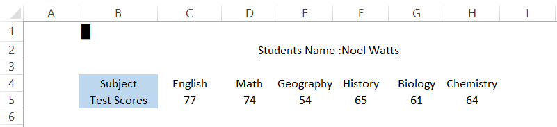
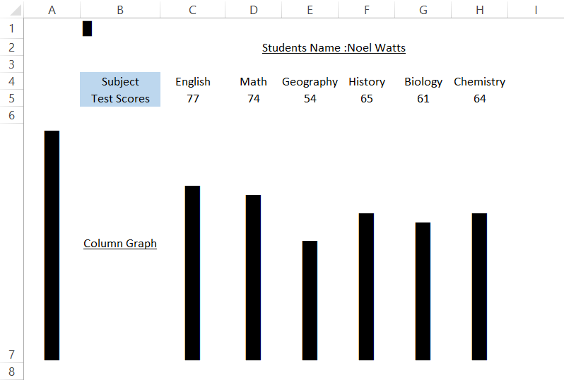
Suppose that you have the test scores for the student as illustrated below:

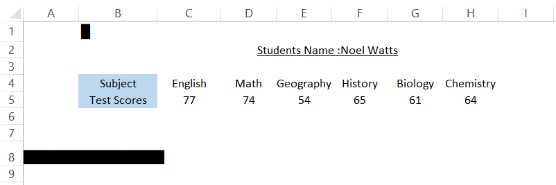
 As usual, we have selected the whole block element from the Arial Black font in cell B1.

Firstly, we want the cells to be sized so they can accommodate the vertical column chart.

We will use the formula =REPT(B1,25) in cell A7, which gives the result:

It doesn't look like a vertical column so far. Next, you need to select cell A4 and change the orientation of the value to 'Rotate Text Up' from the Home tab. You can also use the shortcut key of Alt + H + FQ + U.

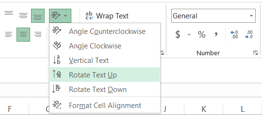
This will give you the result as illustrated below:

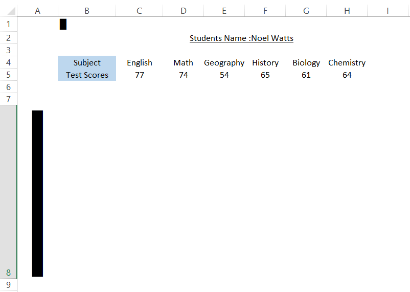
You can later go on and hide column A entirely, but this sets up the cell height for the column chart to work.

Next, you will use the formula =REPT($B$1,(C5-0)/(100-0)*25) in cell C7 and drag it across to cell H7, which gives us the result:

After some more modifications, the final column graph will look as illustrated below:

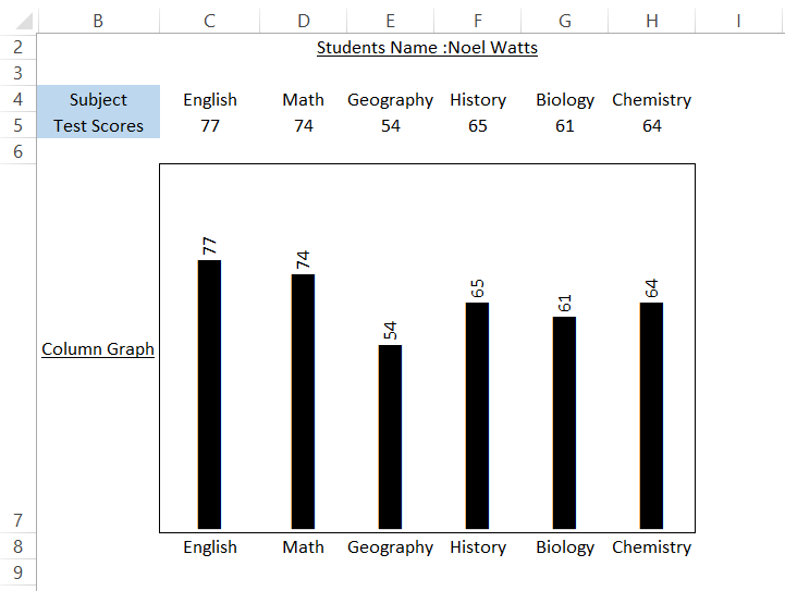
If you are wondering how we added the test scores above the column graphs, then all you need to do is concatenate the test scores in the formula i.e., the procedure will be =REPT($B$1,(C5-0)/(100-0)*25)&" "&C5.

Now, you might have some questions. For example, why was the very first column in cell A7 that we hide 25 repeated characters? But, of course, you can use other numbers too - a large number will create large columns and vice versa.

However, it would help if you remembered that whatever characters were repeated in A7 must be multiplied in the formula we used in cells C7:H7. For example, since we used 25 repeated characters, we multiplied the number_times argument by 25.

If you change any test scores, you will find that the graph automatically adjusts and accommodates those values.

Practical Example of REPT Function

REPT function can also be used to find the position of the 'nth' term within a given text string. That is, of course, in collaboration with other functions in Excel.

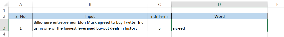
Suppose that you have the text string as illustrated below:

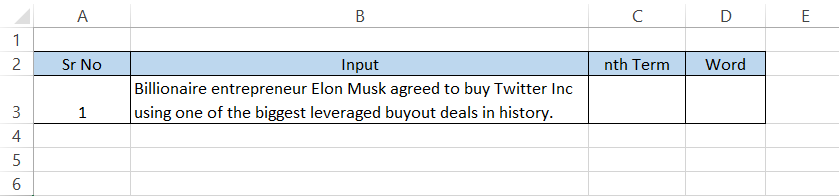
Then, to find the 'nth' term, we will use TRIM, MID, SUBSTITUTE, LEN, and REPT functions.

We will use the formula =TRIM(MID(SUBSTITUTE(B3," ",REPT(" ",LEN(B3))), (C3-1)*LEN(B3)+1, LEN(B$3))), which will give you the result in cell D3 as:

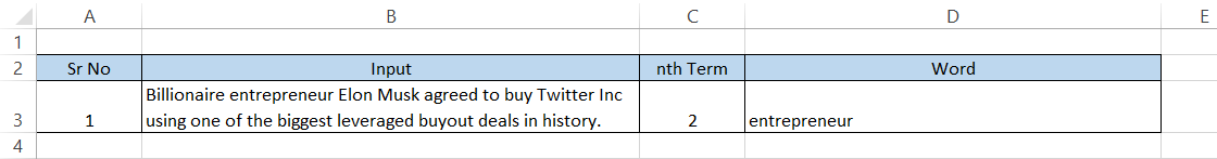
As you can see, when we input the 'nth' term as 2 in cell C3, the formula extracts the second term from our text string.

If you change the 'nth' term in cell C3, let's say to 5, then the result is equal to 'agreed.'

To understand how the function works, let's break it down into several steps:

1. Firstly, the LEN(B3) finds the sentence length equal to 121 characters.

2. The REPT function using the formula REPT("", LEN(B3)) gives space characters 121 times.

3. The formula =SUBSTITUTE(B3," ", REPT("", LEN(B3))) will replace all the single spaces that separate two different words with spaces equal to 121.

4. The result is then enclosed inside the MID function that returns the word based on start_num (the letter from which to return the word) and num_chars (how many letters to return). 

Our  start_num  will be (C3-1)*LEN(B3)+1, where the logic is that each word is separated by 121 spaces, i.e., Billionaire + 121 spaces + entrepreneur, then the start_num directly lands us on our next term. 

The formula so far is MID(SUBSTITUTE(B$3," ",REPT(" ",LEN(B$3))), (C3-1)*LEN(B$3)+1, LEN(B$3)).

5. Even if the word is extracted from the entire string, we don't have to forget the extra spaces we added in our SUBSTITUTE formula. 

Hence, we use the TRIM function, i.e., =TRIM(MID(SUBSTITUTE(B$3," ",REPT(" ",LEN(B$3))), (C3-1)*LEN(B$3)+1, LEN(B$3))). It removes all the additional spaces from the text, which returns the word based on the nth number that you input in cell C3.

Researched and authored by Akash Bagul | LinkedIn

Reviewed and edited by Purva Arora | LinkedIn