RIGHT Function

What is the RIGHT Function?

The RIGHT function in Excel extracts the 'n' number of characters from the right side portion of the text string.

Even though Excel is primarily used as a number-crunching tool, it offers several text manipulation functions to the Excel community. The MID and LEFT function is used mainly to extract text from the middle or left side of the text string, respectively.

Files received from external sources won't always be user-friendly. For example, they may have unwanted characters at different positions, or you might need a particular set of characters rather than the entire text string.

For example, if you are analyzing different real estate properties, i.e., which properties are expensive or cheap based on the zip codes, then that particular information is all you need.

However, 99% of the time, you would find the address in files downloaded from external sources as '99 Street Ave, Buffalo, New York, 10978'. So how would you separate the zip code?

None other than the 'RIGHT function.' In this article, you will understand the function's syntax and explore different examples to help us decipher the part better.

Understanding RIGHT function

The RIGHT is categorized as a text function that will extract a specified number of characters from the right side of the text string.

In another way, you can also say that the function will extract the 'n' number of characters from the ending portion of the string.

For example, if you have the text string as 'Amortization,' you can obtain the ending three characters' ion' as a substring while ignoring all the characters at the beginning of our text string.

The essential component before using the function is knowing how many characters to extract. If you see the position up to which you need the characters, you have already progressed 50% in understanding the function.

In the LEFT function, we count the characters from the beginning of the text string. However, 'things are stranger' for the RIGHT role where the opposite happens.

Here, you count the characters from the end of the text string. The last character becomes 1, and the second last becomes 2, and so on.

Using the count of characters as 3 for 'Amortization,' we can get the result as 'ion' in Excel.

The syntax for the function is:

=RIGHT(text,[num_chars])

where,

• text = (required) the text string from which you intend to obtain the characters
• num_chars = (optional) the number of characters to extract from the text. If you skip the argument, the function takes a default value of 1, meaning it will obtain only one character.

How to use the RIGHT function

There are two different methods with which you can use the function.

a) Method #1: From the function's library

These predefined formulas help you to directly input arguments in the dialog box to get the result in the desired cell. To use the function, please follow the steps below: 

1. Select the cell in which you intend to get the result.
2. Next, click on the Formulas tab > Text > and the function's name.
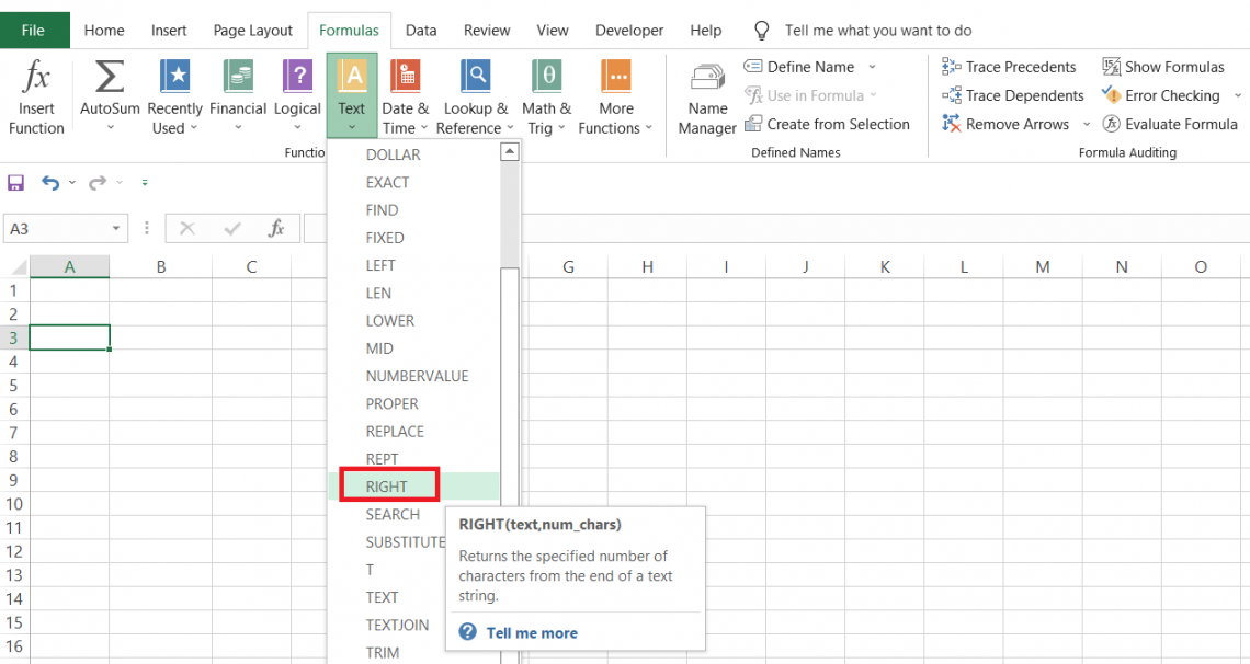
3. This should open up the dialog box, as illustrated below:
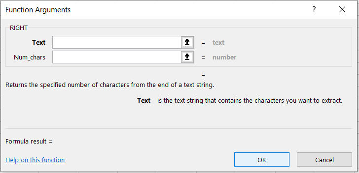
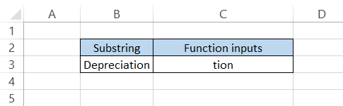
4. Next, we input the arguments in the dialog box. For example, if the text  is 'Depreciation' and the num_chars is 4, then we will get the preview of the result as:
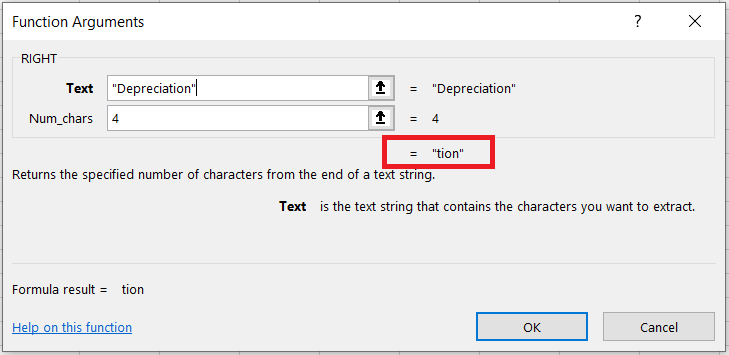
5. If you hardcode the text argument, then you must include quotation marks. You can also directly reference the cell for both views, giving you the same result.
6. When you click on Ok, you will get the result in the selected cell:

b) Method #2: From the function's library

The function can also be used as a worksheet formula, where you begin with an equal sign and input the function name followed by the arguments inside the parenthesis.

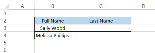
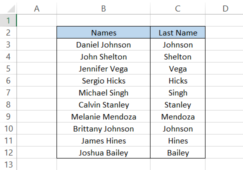
Let's say that you want to extract the last names from the full name of your employees.

To extract the last name 'Wood' in cell C3, we will use the formula =RIGHT(B3,4), which should give you the result:

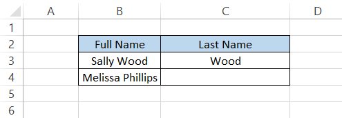
By counting the characters from the text string ending, we conclude that the last name 'Wood' has four characters; hence, the num_chars argument is equal to 4.

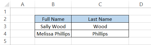
Next on the list is the name' Melissa Phillips.' Can we drag the formula down to get the last word as 'Phillips'? Unfortunately, not! This last name has 8 characters; hence, the num_chars argument would equal 8.

The formula would be =RIGHT(B4,8), which will give you the result as illustrated below:

Changing the formula every time can be a nuisance, so worry not! We have covered a section on separating last names using a 'delimiter' and a SEARCH function. 

Examples Of RIGHT Function

This section will show a couple more examples to understand the function better.

a) Example #1

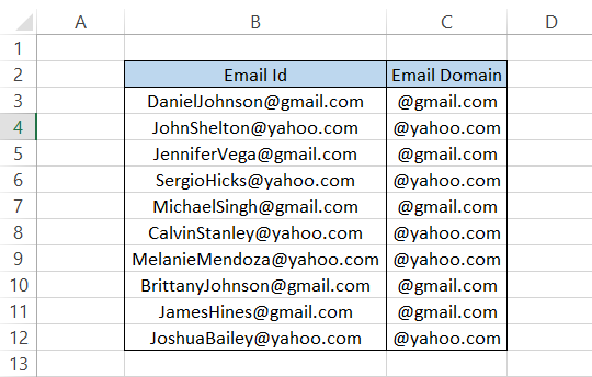
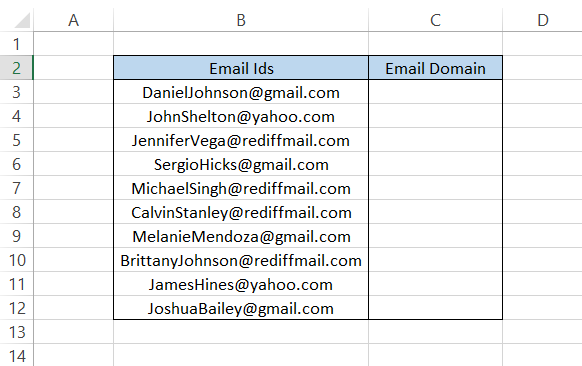
Suppose that you have employee mail IDs in your database, as illustrated below:

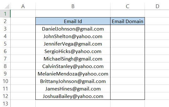
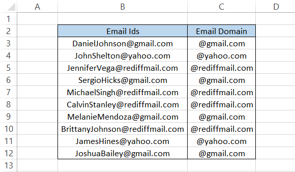
We are glad that both @gmail.com and @yahoo.com have 10 characters each. So, to separate them both in column C, we will use the formula =RIGHT(B3,10), which will give you the result:

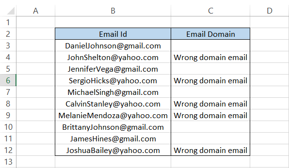
Further, if you want to check if employees only have the @gmail.com domain as their email ID, you can you a combination of the IF function that will evaluate the formula and return two alternative results based on TRUE or FALSE.98+

The formula will be =IF(RIGHT(B3,10)=" @gmail.com,"" ", "Wrong domain email"), which will hide all the correct emails and highlight the wrong domain emails as:

b) Example #2

Suppose you have thousands of rows of data for full names and intend to separate the last words.

You can't just go through all the rows of data, count the characters in the last name, and update the formula individually.

That's where the SEARCH and FIND function comes in.

Both functions have the same syntax:

=SEARCH(find_text, within_text,[start_num])

                        or

=FIND(find_text, within_text,[start_num])

where,

• find_text = (required) the substring that we intend to search for in the text string
• within_text = (required) the text string which will be searched for the substring
• start_num = (optional) the starting position within the text string. For example, if you have the text string as 'DogeCoin' and need to find the position of 'Coin,' we can input the start_num as 1, which should give the position of the sub-string as 6.

Both functions help extract a text string based on a 'delimiter' presence. A delimiter is a character that separates a text substring by forming a boundary between them.

Some of the common delimiters between the text strings are space, commas( , ), semicolons( ; ), a pipe or a vertical line( | ) or the back and front slashes ( / \ )

Returning to our examples based on the names, assume that you have terms of varying lengths from which you need to extract the last words.

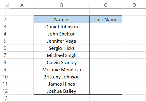
To extract the last names, we will use the formula =RIGHT(B3, LEN(B3)-SEARCH("", B3)), which will give us the result as illustrated below:

How did the formula work? Firstly, the SEARCH function finds the space delimiter in all the text strings. Then, the number obtained is subtracted from the LEN function result.

For example, the length of the Daniel Johnson string is 14, while the space character is present at 7. Subtracting both, we get the result of 7.

Finally, the RIGHT function works magic by finding the substring consisting of seven characters equal to 'Johnson.'

As you can see, even though all the last names are of varying lengths, we can still accurately obtain the substrings. This could only be achieved with the help of a delimiter in the dataset.

c) Example #3

We saw how the email domains could be separated from the employee email ids. But the central assumption was that the substring @gmail.com and @yahoo.com were the same.

What if you have other domains with lengths more or less than others in the dataset?

Suppose you have the employee email IDs as illustrated below:

Then, to separate the email domain, we will use the formula =RIGHT(B3, LEN(B3)-SEARCH("@", B3)+1), which will give us the result:

Now we don't have to worry about the varying string lengths we want to extract from the email IDs.

d) Example #4

Suppose you have a recurring fixed-length substring at the beginning of your text string. How can we remove the first 'n' characters from the series?

Here, you can use the simple combination of the LEN and RIGHT functions.

Let's say the employee data consists of the combination of employee ID and name. However, we do not need the employee IDs and prefer completely removing those before the data is uploaded into the database.

The data looks as illustrated below:

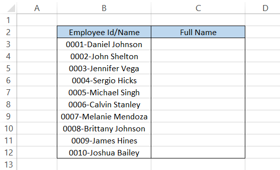
All the employee IDs are made up of five characters - four numbers followed by the dashed ( - ) symbol. 

We know that you have already guessed what we will be doing next.

We will use the formula =RIGHT(B3, LEN(B3)-5), giving us the full name in cell C3 as 'Daniel Johnson.' After dragging down the formula, we will get the result:

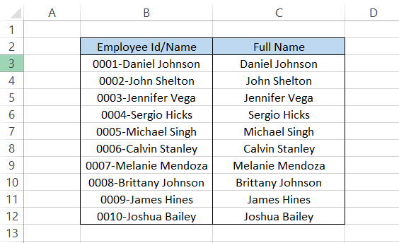
The LEN function finds the length of the entire string from which five characters are subtracted. The result is then used as a num_chars argument in the RIGHT function, which gives us the required result.

e) Example #5

We saw how you could extract the last name from the full name using a simple formula. But what if you also have middle names in some data rows?

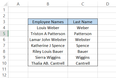
Suppose that the data for the employee names look, as illustrated below:

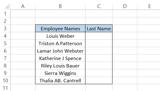
As you can notice, sometimes we do not have a middle name (Louis Weber) or a middle name(Lamar John Webster), while in other instances, the middle name consists only of the initial letter.

In this case, if you use the =RIGHT(B4, LEN(B4)-SEARCH("", B4)) formula, you would only get the wrong results as below:

Apart from cells C4 and C9, all the cells give wrong results. So what formula could be used?

We will use RIGHT, LEN, SEARCH, and SUBSTITUTE functions in such cases.

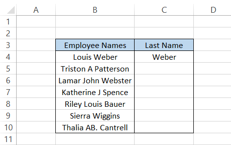
The formula in cell C4 will be 

=RIGHT(B4,LEN(B4)-SEARCH("@",SUBSTITUTE(B4," ","@",LEN(B4)-LEN(SUBSTITUTE(B4," ",""))))),

Which will give you the results as:

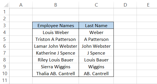
Here comes the moment of truth! Drag down the formula up to the cell C10, which should give you the result as illustrated below:

Exactly the result that we wanted. So how does the formula work? We will try to understand using the Employee name 'Triston A Patterson'

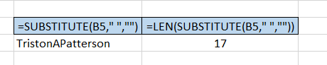
• The formula consists of two SUBSTITUTE functions. The first function in formula =SUBSTITUTE(B5," ","") removes all the space characters. The result is then enclosed inside the LEN function that returns the length of the string as 17.
• Finally, 17 is subtracted from the original text string length using the formula LEN(B5), 19 minus 17, giving us the result of 2.
• The result that we get is an essential component of the formula. Why? Because we will be using it as an instance argument in our following SUBSTITUTE function.
  We take the original text string Triston A Patterson and again substitute the space character with the '@' character BUT! Yes, there is a but to specify that the '@' character is only added at the 2nd space in our text string. 
  So the string 'Triston A Patterson' becomes 'Triston A@Patterson' or the 'Lamar John Webster' becomes 'Lamar John@Webster.'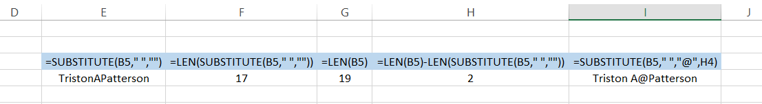
• Finally, the SEARCH function looks for the '@' character inside the newly constructed string and subtracts that number from the length of the entire row. This trims the whole string, including the '@' character. 
• Finally, the number that remains after subtracting the entire string (19) and the position returned using the SEARCH function(10) gives the result of 9.
• The number 9 is picked by the RIGHT function, which replaces the substring as 'Patterson.'
• Every other single last name in the data is produced in the same manner.

Date/Time and RIGHT function

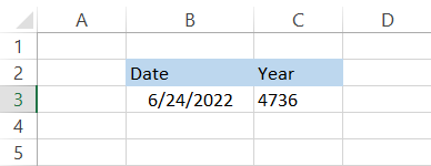
We know that the dates are stored as serial numbers in Excel. So, for example, if the date is 24th June 2022, the serial number corresponding to the date equals 44736.

The dates in Excel begin from 1st Jan 1900, corresponding to serial number 1.

Let's say that we want to extract the year from a date. So naturally, you would expect the result to be something like 2022 or 2023 by using the formula =RIGHT(B3,4).

However, the formula returns a contradictory result which is 4736, which is the last four characters of the serial number 44736.

Extracting seconds or minutes from the time might give deceiving results since even time is stored as a decimal number in Excel.

If you have the time as 11:01:00 PM and try to extract the seconds component from the time using the formula =RIGHT(B4,2), you will get the result as 

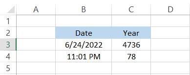
78? But there are just 60 seconds in a minute?

As we said - time is decimal numbers. So when we press the keyboard keys Ctrl + ~, we find that the time 11:01:00 PM is 0.959027777777778, and the last two characters are 78, which is why we get a misleading result.

Researched and authored by Akash Bagul | LinkedIn

Reviewed and edited by Parul Gupta | LinkedIn

Free Resources

To continue learning and advancing your career, check out these additional helpful WSO resources:

• CODE Function
• HOUR Function
• PI Function
• YEAR Function
• YIELD Function