SUMIFS Function in Excel
An Excel Math & Trig function and one of Excel's RACON functions that helps to find the sum of a particular range based on one or more true or false condition(s).


What Is SUMIFS Function?
The SUMIFS Function is an Excel Math & Trig function and one of Excel's RACON functions that helps to find the sum of a particular range based on one or more true or false condition(s).
The SUMIFS provides a flexible way to perform complex calculations by filtering data and determining which cells should be included in the sum. This Math & Trig function was introduced in Excel 2007 and is available in all the subsequent versions of Excel.
This premade function aims to find the sum of the data in a range that meets certain criteria. It can use various operators like:
- Logical Operators like:
- > (greater than)
- > (greater than)
- >= (greater than or equal to)
- < (lesser than)
- <= (lesser than or equal to)
- =(equal to)
- <> (not equal to)
- Wildcards like:
- * (asterisk)
- ? (ampersand)
This function can apply criteria that are based on:
- Texts
- Numbers
- Dates
Instead of using multiple SUMIF functions or manual calculations, SUMIFS simplifies the process by combining multiple criteria into a single formula. This function's beauty lies in its ability to handle complex calculations involving multiple conditions.
This function evaluates each criterion in order and includes only the cells that meet all the specified conditions.
Whether you're analyzing sales data, tracking expenses, or managing inventory, the SUMIFS function can help you extract valuable insights by aggregating data based on specific criteria.
By utilizing the SUMIFS function, you can save time, streamline your calculations, and gain deeper insights into your data by efficiently summing values that meet multiple criteria in a single formula.
In short, the SUMIFS function in Excel is a powerful tool for performing calculations based on multiple criteria. Its versatility, ease of use, and efficiency make it an indispensable function for data analysis, reporting, and decision-making tasks.
- The SUMIFS function in Excel is a Math and trigonometry function used to find the sum of a particular range based on one or more true or false conditions.
- The SUMIFS function returns the sum of the cells specified by sum_range that meet all the selected criteria.
- Each criteria range can contain numbers, arrays, or references that contain numbers. SUMIFS ignores empty cells, text, and cells that contain logical values TRUE or FALSE
- SUMIFS calculates sums based on multiple criteria, such as filtering sales data for a specific product and region.
Syntax of SUMIFS Function
The Syntax for this Function is as follows:

=SUMIFS(sum_range, criteria_range1, criteria1, [criteria-range2, criteria2], …)
Where:
- Sum_range, a required argument, refers to the range of cells to sum. It can be either one or more cells, i.e., it can be a single cell, a named cell, or a range of cells.
- Criteria_range1, another required argument, refers to the range that is supposed to be tested using Criteria1.
- Criteria1, a required argument, refers to the criteria that define which cells in Criteria_range1 will be added.
Note
The Criteria Range and the Criteria form a search pair; after the items in the range are found that pass the criteria, their corresponding values in the sum_range argument are summed up.
- Criteria_range2, an optional argument, refers to the range that is supposed to be tested using criteria2
- Criteria2, another optional argument, refers to the criteria that define which cell in the Criteria_range2 will be added.
Note
Up to 127 range and criteria pairs can be used as arguments.
The Logical Operators can be used in the following ways:
Suppose “a” and “b” are two distinct numbers.
- If a is greater than b, then the argument will be “a > b”
- If a is equal to b, then the argument will be “a = b”
- If a is smaller than b, then the argument will be “a < b”
- If a is less than equal to b, then the argument will be “a <= b”
- If a is not equal to b, then the argument will be “a <> b”
The Wildcard functions like the *(asterisk) and ? (ampersand) can help us find matches that are not exact but similar matches.
The Asterisk (* ) can be used in the following ways:
Suppose there is a number “R”
- *R means that all cells in a particular range that end with R
- *R* means that all cells in a particular range that contain R
- R* means that all cells in a particular range that start with R.
The Ampersand (?) can be used in the following way:
Suppose you know only the first and last letter of a word; let's suppose the word is “fun”, then you will use “f?n”, then it will match with fan or any other letter having f as the first and k as the last letter.
If the data itself has a * or ? Then we use ~ (tilde) in front of the asterisk of the ampersand.
SUMIFS - Example #1
Let's suppose that a clothing company selling Tank Tops in 4 different colors, Red, Blue, Black, and White, has sold these tank tops in 2020, 2021, 2022, and 2023.

We have to find:
- The Profits of White Tank Tops sold in 2021
- The Profits of Blue Tank Tops Sold in 2022
- The Profits of Black Tank Tops sold in 2023
- The Profits of Red Tank Tops sold in 2020
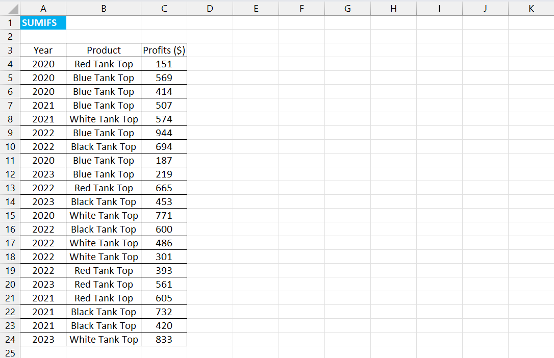
Suppose we have the given data for the Profits of Tank Tops sold over the years.
To find out the Profits of White Tank Tops sold in 2021, we use the following formula as shown in the picture above in Cell G4,
=SUMIFS(C4:C24,B4:B24,"White Tank Top",A4:A24,"2021")
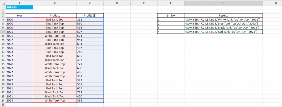
Similarly, we find out the Profits of Blue Tank Tops sold in 2022, we use the following formula in Cell G5,
=SUMIFS(C4:C24,B4:B24,"Blue Tank Top",A4:A24,"2022")
Similarly, we can find out the answers for the Profits of Black Tank Tops in 2023 and of Red Tank Tops in 2020 by applying the formula as shown in Cell C6 and C7.
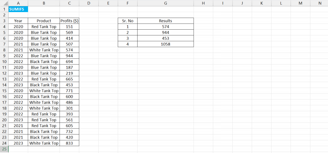
After applying the formulas without mistakes, we arrive at the result above.
SUMIFS - Example #2
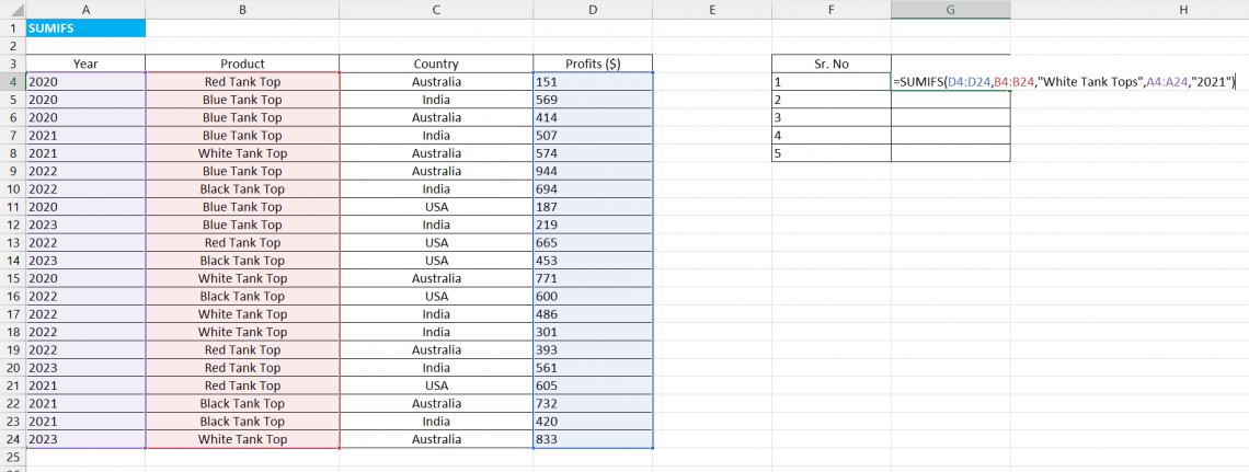
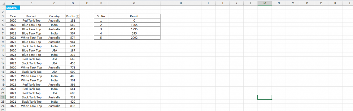
Suppose we get the data in the previous example along with the country of sale; how do we use the SUMIFS Function? This will be answered in this example.
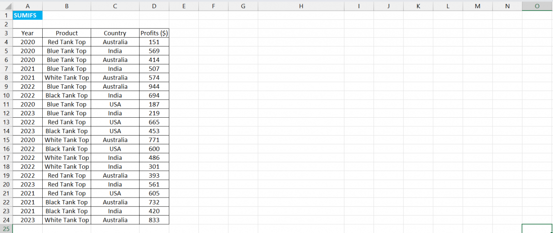
The data, along with the new addition of “Country,” is as above.
Suppose you have to find:
- The Profits of White Tank Tops sold in 2021
- The Profits of Tank Tops Sold in the USA in 2022
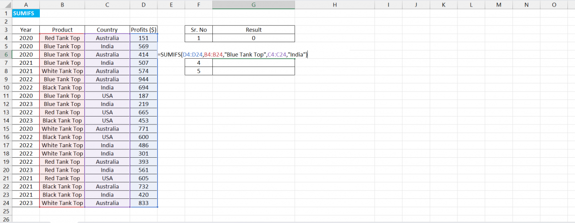
- The Profits of Blue Tank Tops Sold in India
- The Profits of Red Tank Tops Sold in Australia in 2022
- The Profits of Tank Tops sold in 2020.
In the first question, we have to find the Profits of White Tank Tops sold in 2021, we have two criteria:
- White Tank Top Sold, and
- Sold in 2021
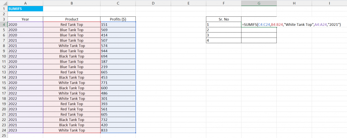
To find out the Profits of White Tank Tops sold in 2021, we use the following formula, which is also shown in the picture above
=SUMIFS(D4:D24,B4:B24,"White Tank Tops",A4:A24,"2021")
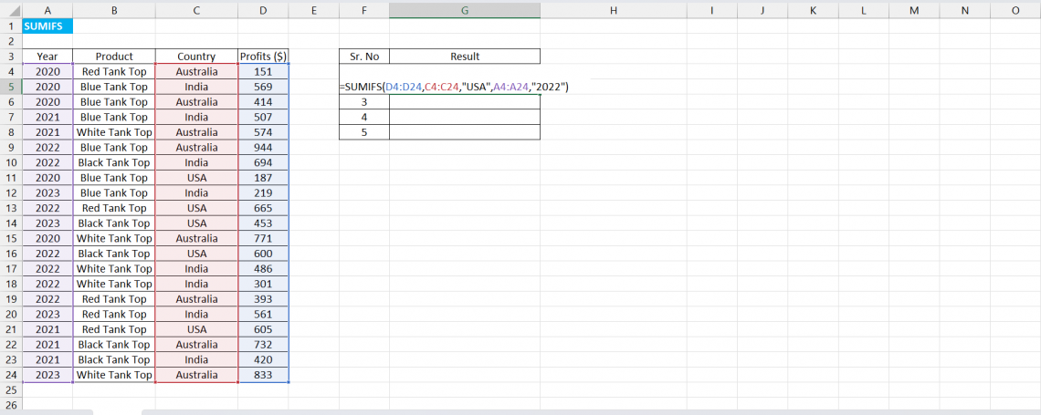
In the second question, we have to find the Profits of Tank Tops sold in the USA in 2022. That means we now have 2 criteria:
- Sold in the USA
- Sold in 2022.
So here, we use a formula similar to the one used in the first question after making appropriate changes, as shown in Cell G5 above.
The third question is to be done similarly to the first and second questions shown above.
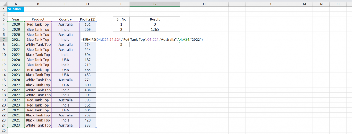
In the fourth question, we have to find the Profits of Red Tank Tops sold in Australia in 2022. Here we have 3 criteria:
- Red Tank Top Sold
- Sold in Australia
- Sold in 2022
So, like in the picture above, we use the Function to achieve the desired results.
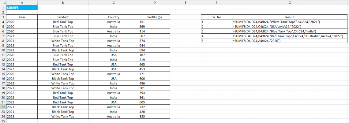
The fifth question can also be done similarly to the first and second questions, as shown in the picture above.
Note
You can check all the formulas in a worksheet by following these steps: Formulas > Show Formulas.
This last step shows all the results of the questions asked. By observing and understanding the 2 examples above, one can easily understand how the SUMIFS Function works in Microsoft Excel.
SUMIFS Function: Points to Remember
There can be other problems that might occur while using this function.

Here are some points you must remember while using this function since it can help you to use it more easily and productively.
- In Excel, we can apply a SUMIFS function on 127 criteria ranges.
- The same length should be used for all the ranges. For example, if the sum_range is A1:A5 and the criterion range is B2:A5, Excel will show a #VALUE! error.
- Operators must be enclosed double quotes, whereas numerical values and cell references shouldn't be enclosed.
- This Math & Trig function works with the “AND” logic, meaning that a cell will only be summed if all the criteria are TRUE. However, we can use another way to sum the cells using “OR” logic by either:
- Using SUMIFS twice
- Using SUMIFS + array constant
- Using Wildcards.
- If the result is Zero (0) instead of the expected result, then one must make sure that the criteria set in the syntax are text values and that they are in quotation marks.
- If the addition of the sum range is incorrect when the range has TRUE or FALSE values, then it is because the TRUE and FALSE values in the range are evaluated differently; TRUE evaluates to 1, and FALSE to 0.
- It is possible to apply wildcard characters like * (asterisk) and ? (ampersand) in the criteria argument. The ampersand helps to match any one character, and an asterisk helps to match any sequence of characters (zero or more).
- If there is an actual ampersand or asterisk, then one can use the sign of tilde (~) like (~?) in the case of the ampersand and (~*) in the case of the asterisk.
- It is important to consider that this Function isn’t case-sensitive; however, one can use a mix of SUMPRODUCT and EXACT Functions to arrive at a satisfactory answer.
- This function requires range; it won't work with an array.
SUMIFS Function In Excel FAQs

These two functions in Excel allow you to sum values based on specific conditions. They serve a similar purpose, several key differences exist between them.
| Criteria | SUMIF | SUMIFS |
|---|---|---|
| Number of conditions | It can evaluate only one condition at a time. You can specify a single criterion to determine which cells to sum. | It can check for multiple criteria simultaneously. You can define multiple conditions to filter the cells that should be included in the sum. |
| Syntax | It can evaluate only one condition at a time. You can specify a single criterion to determine which cells to sum | It can check for multiple criteria simultaneously. You can define multiple conditions to filter the cells that should be included in the sum. |
| Size of ranges |
The sum_range does not necessarily have to be of the same size and shape as the range. As long as the top left cell of the sum_range aligns with the corresponding cell in the range, Excel will adjust the size of the sum_range automatically. |
Each criteria_range in the formula must have the same number of rows and columns as the sum_range argument. If the ranges are not of equal size, a #VALUE! error will occur. |
| Availability | It is available in all versions of Excel, from Excel 365 through Excel 2000. | It is available in Excel 2007 and higher versions. |
If no cells meet the criteria, the SUMIFS function returns 0 (zero).
Yes, you can use cell references for criteria that the user can dynamically change. This allows you to update the criteria without modifying the formula itself.
Yes, you can reference criteria from another worksheet in the SUMIFS function. Simply include the worksheet name followed by an exclamation mark (!) before the range reference.

Free Resources
To continue learning and advancing your career, check out these additional helpful WSO resources:


or Want to Sign up with your social account?