Excel’s Power Pivot
An advanced data modeling and analysis add-in package capable of powerful and sophisticated data modeling and manipulation and establishing extensive relationships and complex calculations.


What is Excel Power Pivot?
Excel Power Pivot is an advanced data modeling and analysis add-in package capable of powerful and sophisticated data modeling and manipulation and establishing extensive relationships and complex calculations.
Power Pivot is an amazing function of Microsoft Excel. Initially introduced in 2010, Power Pivot unlocks new avenues in Excel, tremendously increasing Excel’s capabilities for analysts to undertake heavy resource-intensive tasks efficiently and easily. The Power Pivot is one of Excel's three available data analysis tools:
- Power Pivot
- Power Query
- Power View
Power Pivot brings users crucial insights by implementing key business intelligence functionality into the core of the Excel data and analyzing large volumes of data from various sources.
The key business intelligence functionality includes advanced data modeling and manipulation, a larger capacity than stand-alone Excel spreadsheets, and a powerful formula language known as DAX (Data Analysis Expressions).
Hence, such powerful functionality eliminates extensive workloads and formulas while efficiently transforming large volumes of datasets to produce effective data analysis by the data analysts.
- Excel Power Pivot is an add-in feature available in Microsoft Excel that allows users to import, manipulate, and analyze large datasets from various sources.
- Power pivot can handle complex capabilities, including relationships, intricate calculations (DAX), hierarchies, and Key Performance Indicators (KPIs).
- It enables users to create sophisticated data models, perform advanced calculations, and generate meaningful insights without needing to use complex formulas or pivot tables.
- It unlocks versatility and is useful for Excel users, analysts, and those interested in business intelligence. Pivot effectively utilizes substantial data, relationships, efficient calculations, and data visualization.
Understanding Excel Power Pivot
The Excel Power Pivot, formerly known as PowerPivot (without the space), is a feature of Microsoft Excel that serves as a robust business intelligence (BI) platform for data analysis and modeling. Power Pivot emerged around May 2010 as a separate add-in for Excel 2010.
The Power Pivot can enhance Excel’s local Microsoft Analysis Services capabilities across the workbook by allowing users to build ROLAP (Relational Online Analytical Processing) models, which are not restricted by the workbook and can be done at a core level.
The introduction of Power Pivot is a great relief to the companies. Excel is not ideal for storing data, but for analysis, Excel is awesome. But since the awesomeness is getting restricted by the hit on performance, Power Pivot is a stress reliever.
Unlike workbooks, Power Pivot isn't constrained by workbook limitations. Therefore, it can go beyond the row limit of 1,048,576 since its processing takes internal memory RAM, unlike the workbook, which takes CPU power.
Power Pivot is not just limited to extensive capacity. It can establish extensive relationships between tables and run special DAX (Data Analytics Expression) formula language for extensive data modeling and analysis.
Note
Excel is excellent for extensive data, but opting for specialized software like R programming for massive data is better.
Power Pivot Vs. Excel
This section dives into the strengths and weaknesses of both Excel and Power Pivot to see which works best for a specific task.
| Specific Task | Excel | Power Pivot |
|---|---|---|
| Importing data from different sources. | Available | Available |
| Create tables | Available | Available |
| Edit individual data within tables | Available | Not Available |
| Create relationships between tables | Available | Available |
| Create calculations | Available | Available |
| Create hierarchies | Not Available | Available |
| Create KPIs | Not Available | Available |
| Create Perspectives | Not Available | Available |
| Create PivotTables and PivotCharts | Available | Available |
| Enhancing models for Power View. | Available | Available |
| VBA application | Available | Not Available |
| Group data | Available | Available |
Who Should Use Power Pivot?
There isn't exactly a target audience for using Power Pivot, as Power Pivot is a flexible tool that anyone who deals with data can use. But if we were to generalize potential users, then the main users of the Power Pivot would be:
1. Anyone who is working in an Excel
Individuals who deal with data or use Excel can use Power Pivot to enhance their current data analysis capability. It allows users to work with data more efficiently, providing faster results with less complex formulas and enabling the creation of advanced, auditable models.
2. Anyone who has a taste for Business Intelligence (BI)
Individuals who are interested in Business Intelligence can benefit greatly from Power Pivot. It is considered a stepping stone into Business Intelligence since both share common traits such as data modeling and connecting data for analysis.
Therefore, users or analysts who know Power Pivot have excellent transferable skills, such as Data Modeling and DAX, which are needed in Business Intelligence tools such as Power BI.
When to Use Power Pivot?
There is no specific time to use Power Pivot; anyone at any time can take benefit of the Power Pivot. However, its true potential becomes evident when encountering certain data-related challenges in Excel. Below are some pointers when it is time to shift:
1. Exceeding row limitation
In Excel, there is a limitation on how much data can be pulled. To be exact, Excel (2007 versions onward) only has 1,048,576 rows and 16,384 columns. And to add some salt to the wound, the Excel shows signs of wear out by the 100,000th entry.
The limitations of rows and columns and the instability Excel provides beyond a point are perfect indications to shift to Power Pivot.
2. Relating data
Excel is a key program for performing data manipulation and analysis. Connecting data to perform a calculation is a crucial part of data analysis such that functions like Vlookup, Xlookup, Index, and Match are heavily utilized.
However, dealing with massive data exceeding a couple of millions of rows is quite an extensive task for Excel. For each cell, a formula needs to be processed each time any changes are incorporated into the model. It is quite CPU-intensive.
This is where Power Pivot shines, as Power Pivot has the function of creating a simple relationship between data called a Data Model. Data Model can be deployed when needed, i.e., formulas can be reduced, and constant updation is eliminated.
This leads to less resource utilization, efficient productivity, and fewer errors, which are prone to massive formula extensive tasks.
3. Filtering Data
Power Pivot seamlessly integrates with Excel's Pivot tables, allowing for efficient data filtering and sorting.
With the massive data being efficiently optimized, decisions can be made by procuring insights and visualization of not just any data but specific ones. The Pivot table does exactly that, filtering the useful data.
4. Dealing with resource-intensive functions
The Power Pivot has a powerful function of measuring using DAX language. Measures act as specialized functions that can be applied to specific tables without affecting the entire dataset.
Take an example of a time metric when manipulating an employee’s table to understand each employee’s age. Typically, an analyst would use the Excel time function on the whole table by creating a separate column, “Age.”
This is a resource-intensive task; any further adding or updating the table, Excel recalculates the Age column again. Now, using Power Pivot, you can create a separate measure for Age without adding anything to the original dataset.
5. Variables
It is uncommon not to see nested formulas while using Excel, especially since they reduce workload later in the model. However, the issue is that it is quite hard to understand who is trying to maintain or perform an audit from a third-person perspective.
This is where Power Pivot has an advantage. Power Pivot leverages DAX language. The special feature of DAX is that it needs assigned variables in which intermediate values are stored.
Even though it may be an additional task, it can save time in the long run. Excel has functions similar to DAX, such as LET, but they are nowhere near the DAX experience.
How To Use Power Pivot?
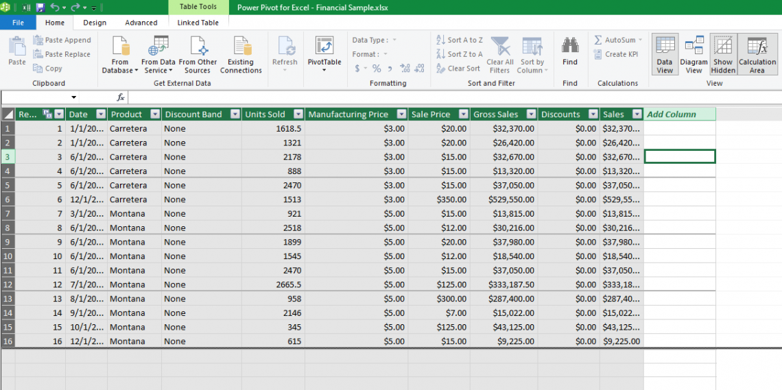
In this section, we will explore “how” to get started with Microsoft Excel Power Pivot. For the demonstration, we have used the Excel data sample Financial Sample from Microsoft.
The following steps apply to Microsoft Excel 2013 onwards and Microsoft 365.
Getting Started With Power Pivot Add-In
To get started, we would have to install Power Pivot in Microsoft Excel. As mentioned, Power Pivot comes as an add-in, and Excel 2003, 2016, and 365 have an in-package COM Power Pivot add-in. The installation is a one-time process.
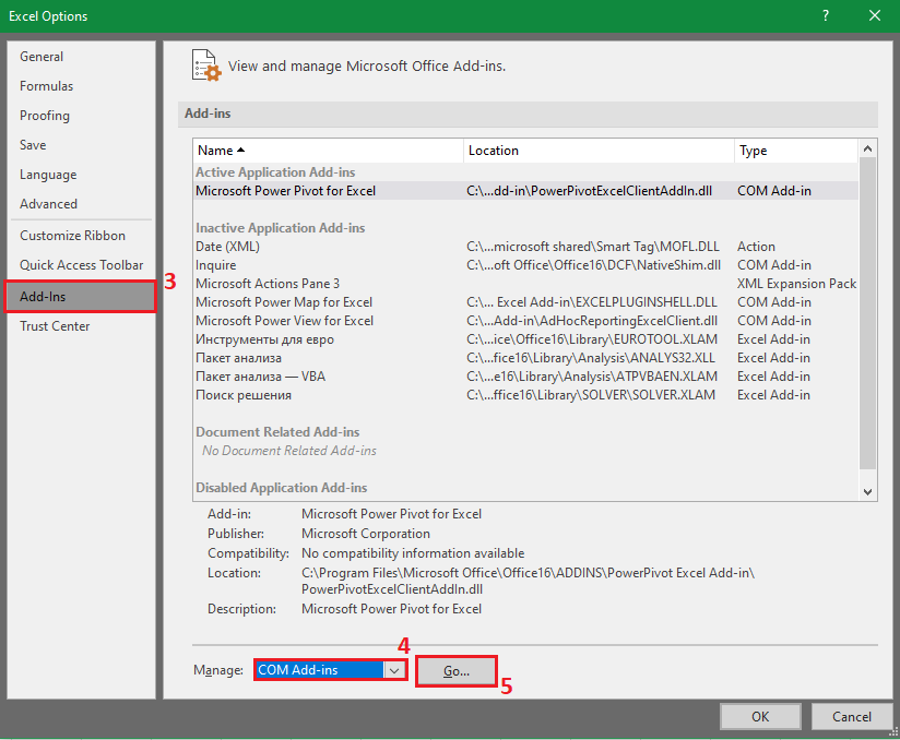
To install the Power Pivot add-in
Step 1: Click on File.
Step 2: Select Options.
Step 3: Within Options, Select Add-Ins.
Step 4: Under the Add-Ins section, select “COM Add-ins” from the Manage droplist.
Step 5: Select Go.
Step 6: Select the “Microsoft Power Pivot for Excel” checkbox.
Step 7: Select OK.
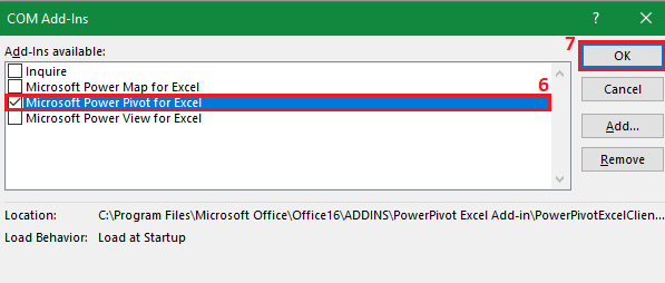
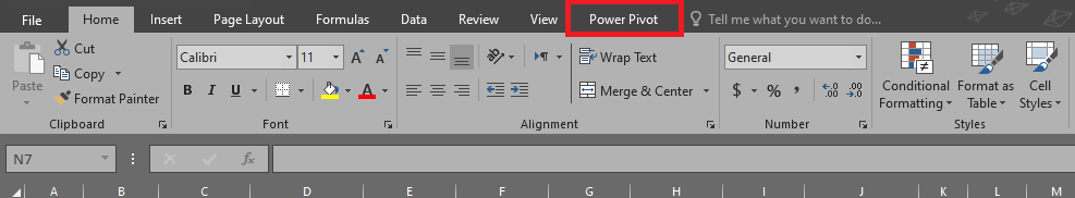
After completing the above procedures, the Power Pivot should appear in the Excel Ribbon.
Note
The above procedures are similar across the versions of Microsoft Excel from 2013 onwards. Users of Microsoft Excel 2010 should download Power Pivot Add-In from the Microsoft Site.
Importing Data Into The Power Pivot
Now, we can start importing data for manipulation and analysis. This section only shows how to import data; no manipulation or analysis is further discussed.
Often, companies draw data from Excel, especially if the company is a small-sized company, whereas, for medium to large-sized companies, the data is often pulled from a Relational Database Management System (RDBMS) like Microsoft Access or Microsoft SQL Server.
The sources for data are plenty, and there are several ways to import data from different sources in Excel.
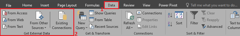
To import data:
Step 1: Click the Data in the Ribbon.
Step 2: Select any of the options within the block called “Get External Data” to import data from different sources.
Note
You can also import external data from New Query, which is much easier when importing Excel files, and it can be found within “Get & Transform” under Data Ribbon.
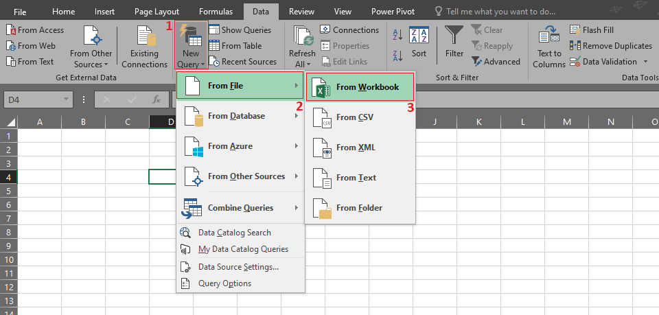
The recommended method for importing data is to use Power Query via New Query. Power Query is an in-built Excel tool that simplifies the user’s efforts in importing and transforming data, which can then be used for Power Pivot.
Power Pivot via Power Query makes any updation to the main dataset a quick fix with a single click. Here's how to import data using Power Query:
Step 1: Select New Query from the Data Ribbon's Get & Transform section.
Step 2: Select From File.
Step 3: Select From Workbook.
Step 4: Select the file.
Step 5: Click Import.
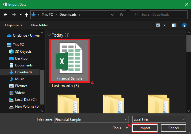
A file preview window appears.
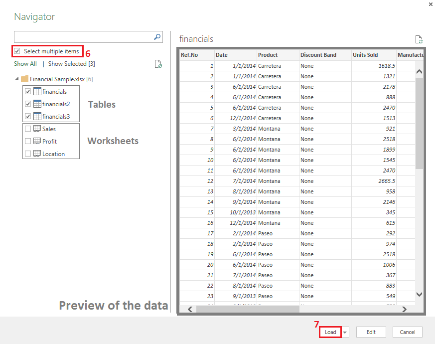
Step 6: If the file has only one table, then click the table.
But if there is more than one table, click the “Select multiple items” checkbox and select the interested table or (if needed) a worksheet.
Step 7: Click load.
After loading the data, the Power Query Editor will be opened, from which further data manipulation and analysis can be performed using many tools provided by the Query Editor.
The Power Query Editor has numerous tools and functions that tremendously aid data analysis.
Creating The Data Model
The next step would be to create a data model for each table in the dataset. The data in the data model stays in the dataset as long as it's not removed. Therefore, you can visit the model whenever you need to.
To create the data model
Step 1: Open the imported Excel file.
Step 2: Convert the data into a table if the data is not tabularized.
Step 3: Make sure that the cell selected is within the table.
Step 4: Open the Power Pivot ribbon
Step 5: Click Add to Data Model within the Tables section.
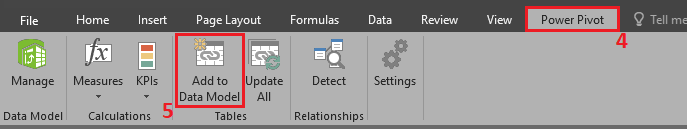
Now, the data has been successfully added to the Data Model. The editor should look similar to what is shown below. This is the default view setting in Power Pivot, as sophisticated data modeling and manipulation takes place without affecting the main dataset.
Note
Click “Manage” under the “Power Pivot” ribbon to open an existing data model. Click “Update All” under the “Power Pivot” ribbon to update any data model.
Creating Relationships
Till now, we have learned to install Power Pivot, import data, create a Data Model, open the created Data Model, and update the Data Model. Now, we can explore a feature in which Power Pivot excels in Excel—got the joke?
This powerful feature is none other than connecting the tables or the relationship between the tables, whichever you want to call it.
Power Pivot leverages by creating separate relationships between the tables to minimize resource use. At the same time, the output is maximized so that the whole dataset is not affected.
Now, let’s see how it's done.
Relationships between tables are created by the simple process of Drag and drop. The columns in a table are used to connect different tables. This method is much easier than typing in formulas and such.
Note
When connecting tables via columns, the values in the column should be of Distinct values only, i.e., unique values, and should contain any repeated values, and the relationship can be created using the “Diagram View” and not the “Data View.”
With the above in mind, there are two types of columns
- The data or The Fact Table (in SQL terms, this is the Primary Key)
- The Lookup or The Dimension Table (in SQL terms, this is the Foreign Key)
For example, in the Financial Sample dataset, we have three worksheets: Sales, Profit, and Location, each containing a table and a Ref.No column with unique, non-repeating values. This makes it an ideal column for connecting tables.
The connection is made by dragging and dropping the distinct column (Ref.No) of the primary (Sales) worksheet onto the secondary (Profit and Location) worksheet, which represents the primary worksheet.
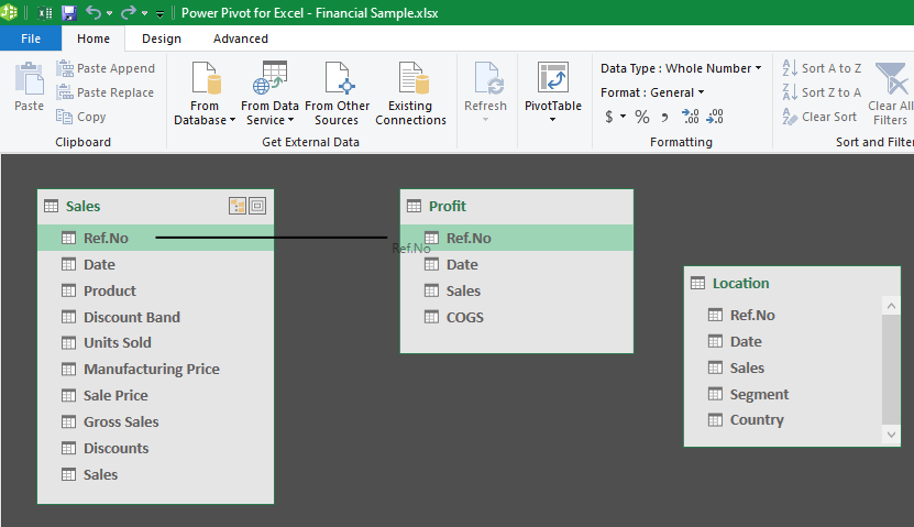
The connection of the diagram is as follows:
- Sales are the primary worksheet
- Profit and Location are the supportive (secondary) worksheets.
Understanding the analogy of the worksheet can help analysts understand how the data flows to accurate data retrieval and better data storytelling. From this point onwards, the analyst gets a better grasp on how to connect the tables.
Therefore,
- Sales Ref.No connects Profit Ref.No.
- Sales Ref.No connects Location Ref.No.
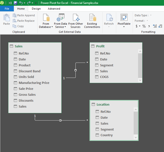
Knowing which table retrieves the data and which table it gets retrieved from is essential. Understanding the data flow can help retrieve the right data. To identify which table connection (or relationship) is of which type. Observe the endings of each connection line.
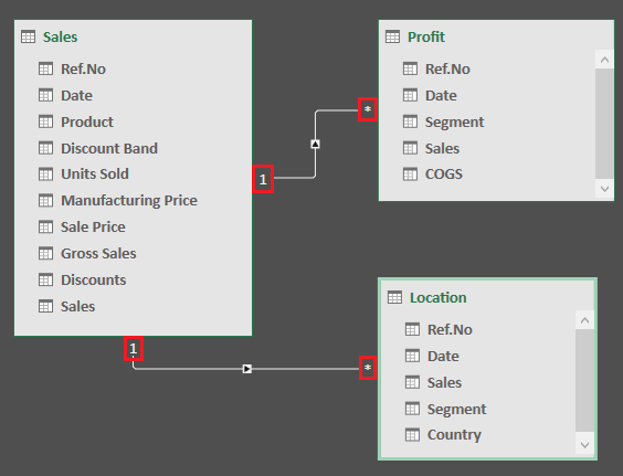
At the end of each connection line, there is an indication
- 1 indicates the primary column retrieving the data.
- Asterisk (*) indicates the data being retrieved from multiple columns in this table.
Note
Unlike the BI tools or programming language, which has One-to-Many, Many-to-One, and Many-to-Many types of relationships, the Power Pivot only possesses a One-to-Many relationship type, in which a table retrieves data from multiple columns from another table.
What Is A DAX?
One might be wondering, “What is this DAX thing this guy is blabbering about?”.
Well, DAX, an abbreviation for Data Analysis Expression, is a formula expression language used for custom dynamic calculations. It was developed by a team of SQL Server Analysis Service at Microsoft as part of Project Gemini, which was released in 2009.
Thus, the DAX language became a native feature of Microsoft services such as Power Pivot, Power BI, and SSAS tabular models.
DAX formula has two distinct types of calculation:
1. Calculated Columns
A Calculated column is a DAX feature used to create additional columns that perform specific functions in the Data Model and can be later used in the PivotTable functions.
Note
The best practice for the calculated column is to implement it within the original dataset or the Power Query Editor instead of the Data Model, as such columns can become essential insights when dealing with further data drills.
2. Calculated Fields (also known as Measures)
A Measure is a query definition (DEFINE) of the calculations in a DAX model. The measure defines whatever calculations are specified regardless of any original dataset formulas. The unique part is that it runs when needed, making it resource-efficient.
The difference between the calculated column and the measure is that the calculated column is Table-specific, whereas the measure is Model-specific.
To learn more about Excel Power Pivot, utilizing Microsoft's free resources is highly encouraged.
Excel Power Pivot FAQs
Power Pivot is an Excel add-in that is used to create sophisticated and advanced data models and relationships for data manipulation and analysis.
The main difference between Power Pivot and normal Pivot is that normal Pivot lists out a table with the chosen data fields, whereas Power Pivot allows users to access the fields within the listed data model and perform analysis based on any related tables.
Data Analysis Expression (DAX) is a formula language used to perform custom calculations for Calculated Columns and Calculated Fields, i.e., Measures.
YES! Power Pivot is a free add-in feature available for all Excel users.
Power Query is a tool used to produce a simple large set of data for analysis. In contrast, Power Pivot is a tool used to create more powerful models and calculations.

Free Resources
To continue learning and advancing your career, check out these additional helpful WSO resources:


or Want to Sign up with your social account?