Amortization Schedule
A table designed to keep track of periodic payments for amortizing loans.


What Is An Amortization Schedule?
An amortization schedule is a table designed to keep track of periodic payments for amortizing loans. It summarizes how much is paid each period. This payment is divided between paying off the principal and paying interest on the loan.
Usually, the debtor pays a fixed amount every period until the loan is paid off. This payment is split between paying for the principal amount (the size of the loan arrangement) and paying interest on the loan.
Naturally, during the first payments, a large portion of the periodical payments would be dedicated to interest. That’s because the principal amount is initially large.
Progressively with each period, the amount paid as interest would decrease, and the amount paid for the principal would increase until the principal is paid off completely.
These schedules are essential for businesses and people who want to estimate their costs and expenses throughout the life of the loan. It also lets them find out how much money paid for interest can be saved if they decide to pay more in the future.
Setting an amortization schedule can be done quickly by using an amortization calculator. However, it can also be set up by manual calculations. Therefore, it is helpful to be familiar with how the numbers are calculated, as it will help you to understand the foundations of taking out a loan.
There are several main types of amortization schedules. Each variety uses a different method to amortize a loan. The main techniques are:
- Straight line,
- Fixed-rate (annuity),
- Declining balance,
- Balloon Payment,
- Bullet Payment,
- Negative amortization.
Amortizing a Loan
Amortizing a loan is a way to repay a debt by periodic - although not necessarily equal - payments. This method requires you to pay interest and a portion of the principal with each regular price.
The principal of a loan is the initial size of the loan that was arranged. It is also called the face value of a loan, used mainly in notating bonds. With the last loan payment, the principal amount of the loan must be fully paid off.
The interest, on the other hand, is the sum of money gradually paid for the service of borrowing the principal. The interest payment is dependent on the interest rate.
The higher the interest rate, the higher the amount of interest paid. Interest rates are usually quoted as annual rates.
As mentioned, the amount of interest paid each period will decrease. That is because paying the appeal is based on the amount of top left.
By gradually paying off the principal, the size of the principal left to pay will decrease. Hence, interest payments will generally decrease over the life of the loan.
It is important to note that the first payment is made at the end of the first period of the loan unless stated otherwise. The size of the last amount, which ultimately repays the debt, can slightly differ from the earlier payments.
The amortization of a debt is completed when the entire principal is paid off. This can include different types of debt and debt instruments, including:
- Loans (personal loans, car mortgages, home mortgages),
- Bonds,
- Promissory notes,
- Debentures
The detailed forecast of costs and expenses throughout the life of the loan is an essential aspect of these types of debt. They accurately list the amount of principal to be paid, the interest expense for that period, and the total outstanding balance that needs to be paid.
Preparing a loan amortization schedule
As mentioned, amortization schedules are helpful as they include a detailed description of the loan repayment. Such tables usually have multiple rows and columns representing the different variables and parameters.
Usually, the rows of the scheduled show for which period the payments presented belong. Periods are typically quoted in months. The number of rows in the table depends on how many periods are allocated to pay off the debt.
Meanwhile, the different columns in the table summarize the other balances and payments to be made.
The columns usually include:
- the beginning balance (which is the outstanding loan balance)
- the total payment to be made for that specific period
- the interest expense
- the principal paid within that particular period
The interest expense is calculated by multiplying the beginning balance by the annual interest rate. For example, if the loan is amortized monthly, the annual interest rate must be divided by 12 to calculate the interest expense.
The interest expense and the principal paid in a specific period together make up the total payment in a single period.
Sample amortization schedule
Below is a schedule that includes all the necessary elements of amortizing a loan.
| Year | Beginning Balance | Total Payment | Interest Paid | Principal Paid | Ending Balance |
|---|---|---|---|---|---|
| 1 | 5,000 | 1,450 | 450 | 1,000 | 4,000 |
| 2 | 4,000 | 1,360 | 360 | 1,000 | 3,000 |
| 3 | 3,000 | 1,270 | 270 | 1,000 | 2,000 |
| 4 | 2,000 | 1,180 | 180 | 1,000 | 1,000 |
| 5 | 1,000 | 1,090 | 90 | 1,000 |
0 |
| Totals | $6,350 | $1,350 | $5,000 |
In this simplified schedule, we can first see that the payments are made annually. Then, looking at the principal paid column, an equal amount of principal is born yearly.
Since the initial principal amounts to $5,000 over five years (which means that $5,000 is being borrowed), the borrower must pay 5,000/5 = 1,000 dollars every year, in addition to interest.
As mentioned, the interest paid is found by multiplying the beginning balance by the interest rate. Supposing the interest rate is fixed at 9%, the interest expense of the first period (the first year) should be equal to $5,000 * 9% = $450.
Notice that the size of the yearly interest expense is decreasing. That is because part of the principal is being paid off with time; hence, interest paid each year will be less than the previous one.
Once we find out the principal payment and the interest expense for a certain period, adding both figures will give us the total payment for the loan.
For example, in year 1, the payment for the principal is 1,000 (as with every year), and interest expense is equal to $450. Therefore, in a year, the total payment for the loan amounts to: 1,000 + 450 = $1,450.
Because payments for the principal are uniform throughout the life of the loan, and interest payments are decreasing with every year, the annual revenues of this specific loan will decrease every year.
This is a crucial characteristic of the amortization method called the straight-line method. Repaying equal amounts of the principal will decrease yearly payments over time. The upcoming sections will discuss other methods of preparing such schedules.
Another important aspect of loan amortization schedules is that the ending balance of one period is the beginning balance of the following period, as seen in every period in the table above.
This is why such schedules are essential for budgeting and organizing loan payments. Using this table, any borrower would quickly know how much they still owe, how high the following cost is, and what percentage of that payment is in the form of interest.
Anyone can easily prepare these schedules with software like Microsoft Excel.

Amortization table using the fixed rate method
The fixed-rate method is a way to pay off the debt in the form of an annuity. The debtor borrows a certain amount of money (the principal) with assistance. Still, the periodic payments are always equal throughout the life of the loan, unlike the straight-line method.
This way of repaying debt is also known as equal monthly installments, where all installments (payments) are similar to each other. Note that this also works for annual costs.
As always, the interest expense will decrease with every period because the size of the top left is decreasing.
However, since the size of the payments is equal, this means that as interest expense decreases over time, the amount paid for the principal will increase to maintain the same amount of periodic payments.
One of the key differences between this method and the straight-line method is that in this method, the principal paid each period increases with each installment. In the straight-line method, equal amounts of principal were paid each period.
The fixed-rate method is most commonly used for repaying large loans, such as home mortgages and car loans. That is because it will be easier for the debtors to repay the loan with fixed monthly payments.
Calculating the monthly payments is slightly more complicated in this method, as we have to find the size of the periodic payment by using a specific formula:
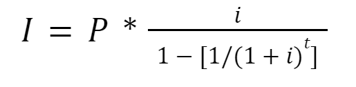
Where I represents the periodic installment (monthly or yearly), P represents the principal (the amount borrowed), i represents the interest rate (needs to be divided by 12 if installments are monthly), and t represents the number of payments.
Example of amortization schedule using the fixed rate method
For simplicity, we are taking the same example as we did previously. $5,000 is borrowed at a rate of 9% and needs to be paid back in five years with annual installments. By using the fixed-rate method, we need to find the amount of the yearly payments. By using the formula:
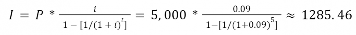
Therefore, each year, $1285.46 will be paid. This amount is distributed between payments for the principal and interest payments. The schedule will look as follows:
| Year | Beginning Balance | Total Payment | Interest Paid | Principal Paid | Ending Balance |
|---|---|---|---|---|---|
| 1 | 5,000.00 | 1,285.46 | 450.00 | 835.46 | 4,164.54 |
| 2 | 4,164.54 | 1,285.46 | 374.81 | 910.65 | 3,253.88 |
| 3 | 3,253.88 | 1,285.46 | 292.85 | 992.61 | 2,261.27 |
| 4 | 2,261.27 | 1,285.46 | 203.51 | 1,081.95 | 1,179.32 |
| 5 | 1,179.32 | 1,285.46 | 106.14 | 1,179.32 | 0.00 |
| Totals | $6,427.31 | $1,427.31 | $5,000.00 |
We already know how to find the total payment by using the formula. The total price is divided between interest payment and principal payment.
To calculate the interest payment, multiply the beginning balance by the interest rate (9%). Finally, the principal payments will equal the total paid minus the interest expense.
A couple of significant differences can be noticed between this table and the one using the straight-line method:
- The total interest paid in the fixed-rate method ($1,427.31) is larger than the genuine interest paid in the straight-line method ($1,350). At the start of the loan, the principal payments are smaller in the fixed-rate form than in the straight-line method.
- Total payments made in the fixed-rate method ($6,427.31) are more significant than the total payments made in the straight-line method ($6,350). That is because of paying more interest in the fixed-rate form.
Therefore, using the fixed-rate method requires the borrower to repay the loan somewhat more slowly. This will result in a larger final total payment, yet it is more straightforward for long-term mortgage holders to use.
Amortization table using the declining balance method
The declining balance method is another method of amortizing a loan. It is pretty similar to the straight-line method but only more fast-paced. That is because the amortization rate determines the principal payment for each period.
Rather than paying equal principal amounts each period, the borrower will pay a predetermined percentage of the outstanding balance.
This percentage is called the amortization rate. Each period, the principal payment will equal the amortization rate multiplied by the outstanding balance.
As always, the interest expense will equal the interest rate multiplied by the outstanding balance. Adding the interest expense and the principal payment will yield the total income for a specific period.
The principal payment will be much more prominent during the loan's beginning than the ending periods. After all, the amortization rate is a fixed percentage. Hence every time a portion of the principal is paid, the following principal to be paid in the next period will be smaller.
Whenever more principal is paid in the earlier stages of a loan (as in the declining balance method), the interest expense will be pretty low throughout the life of the loan. This is the main advantage of the declining balance method.
One disadvantage of this method which was already discussed is that it requires large amounts of principal payments in the first periods. This idea is rather contradictory to the idea of taking out a loan, which can make debt repayment by using this method quite unattractive.
Example of amortization schedule using the declining balance method
For simplicity, we are taking the same example as we did previously. $5,000 is borrowed at a rate of 9% and needs to be paid back in five years with annual installments. Suppose the amortization rate is 40%.
This means that for the first year, the principal paid will amount to $5,000 * 40% = $2,000. The schedule will look as follows:
| Year | Beginning Balance | Total Payment | Interest Paid | Principal Paid | Ending Balance |
|---|---|---|---|---|---|
| 1 | 5,000 | 2,450 | 450 | 2,000 | 2,000 |
| 2 | 3,000 | 1,470 | 270 | 1,200 | 1,800 |
| 3 | 1,800 | 882 | 162 | 720 | 1,080 |
| 4 | 1,080 | 529.2 | 97.2 | 432 | 648 |
| 5 | 648 | 706.32 | 58.32 | 648 | 0 |
| Totals | $6,037.52 | $1037.52 | $5,000 |
The way to find the interest expense and total payment remains the same. In year 5, we didn't have multiple outstanding balances, which was $648 by 40%. That is because the loan matured in year 5, so we wrote off whatever remains in the due compensation to the principal paid column.
The declining balance method resulted in the smallest amount of total interest paid among the three ways. In addition, most of the principal was delivered in the first couple of periods, significantly reducing the interest expense for the upcoming periods.


or Want to Sign up with your social account?