ACCRINTM Function
A Financial function in Microsoft Excel that helps determine the accrued interest for a security that pays interest at maturity.

What Is ACCRINTM Function?
The ACCRINTM Function is a Financial function in Microsoft Excel that helps determine the accrued interest for a security that pays interest at maturity. The word “ACCRINTM” represents “Accrued Interest at Maturity.”

The maturity date refers to the end of a bond's term. Some securities interest periodically or all at once. Once the bond is exhausted, it will return the total interest paid on its face value to the broker or company.
The ACCRINTM function is categorized under the Financial Function in Microsoft Excel and was introduced in the 2007 version of MS Excel. There are two functions that return the accrued interest: the ACCRINTM and the ACCRINT functions.
- The ACCRINTM function, available in spreadsheet software like Excel, is used to calculate the accrued interest for a security that pays interest at maturity.
- The function is commonly used in bond valuation and investment analysis to determine the accrued interest that investors are entitled to receive when purchasing bonds between interest payment dates.
- The syntax for the ACCRINTM function includes arguments such as issue date, settlement date, coupon rate, face value, and optional day count basis.
- The ACCRINTM function can be integrated into financial models and spreadsheets to automate interest accrual calculations for various securities and investments.
Why is ACCRINTM used?
In finance, bond prices are quoted as "clean." No interest due since the issue date or any subsequent coupon payment shall be considered in the "clean price" of a bond.

The price, including accrued interest, is the "dirty price" of a bond. It can calculate accrued interest for a bond that pays periodically at maturity (i.e., only pays interest once).
This function is particularly relevant for investors and financial analysts who must be able to determine the income gained from investing in bonds or securities.
So, what's the difference between these two?
The ACCRINT Function helps determine the periodic interest payments by the issuer. In contrast, the ACCRINTM Function helps to find the total or the lump sum interest payment paid by the issuer on the maturity date.
Hence the Extra M stands for Maturity at the end of the ACCRINTM function.

The Syntax for the ACCRINTM function is given as
=ACCRINTM(issue, settlement, rate, par, [basis])
Where,
- Issue: a required argument; refers to the date on which the security is issued.
- Settlement: another required argument; refers to the date on which the security gets settled, also known as the Settlement date or Maturity Date.
- Rate: a required argument; refers to the annual (yearly) coupon rate of the issued security.
- Par: a required argument; refers to the face (par) value of the security; in the absence of any arguments in this, the function will automatically use $1,000 as the par value.
- Basis: the optional argument in this function; refers to which type of day count will be used in the calculation of accrued interest of the security.
This function returns a positive real figure expressed in the same currency units used to determine the par value of the securities, which is the accrued interest.
NOTE
When one uses the ACCRINTM Function, it is assumed that the interest will only be paid on maturity. If you want to calculate periodic installments of payments, you must use the ACCRINT Function.
The following table refers to the day count basis, which will be used by omitting or entering a number between 0 and 4.
| Basis | Day count basis |
|---|---|
| 0 or omitted | US (NASD), which is 30/360 |
| 1 | Actual/actual |
| 2 | Actual/360 |
| 3 | Actual/365 |
| 4 | European, which is 30/360 |

Example of ACCRINTM in MS Excel
We just discussed the syntax and components of the ACCRINTM Function in Excel; now, let's have a look at some examples to understand how the function works in Excel.

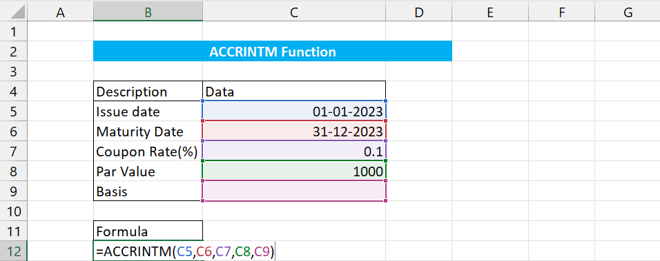
Example 1: DATE Function & Referencing.
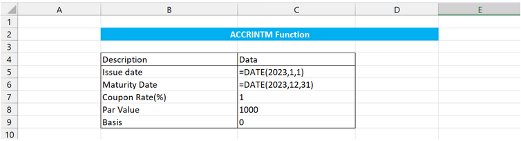
Let's have a look at the data provided in the first example.
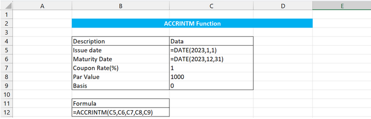
Here, it can be seen that the arguments won't be hardcoded; rather, they will be referenced to cells C5, C6, C7, C8, and C9.
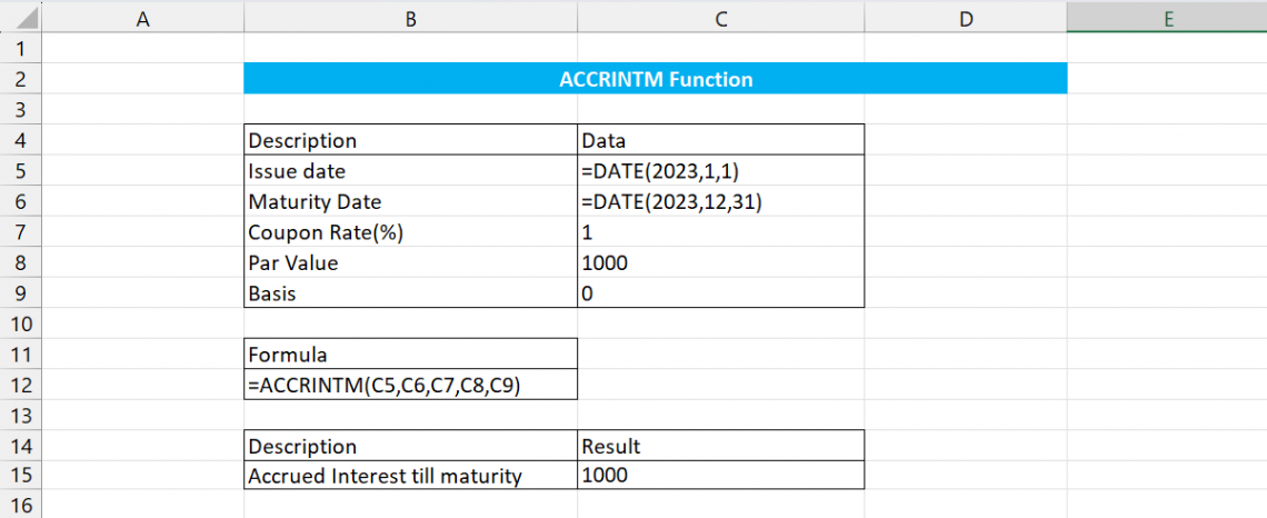
Finally, after referencing the cells, we achieved the result, which is 1000.
Example 2: Absent Value of Basis & Referencing
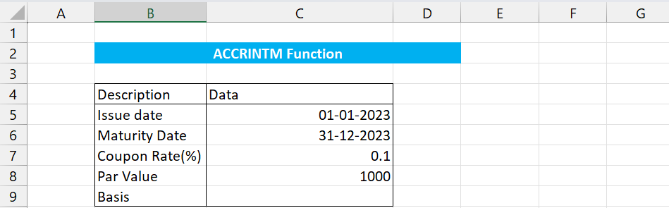
In the second example above, we have formatted cells C5 & C6 by
Select Cell C5 and C6 > CTRL + 1 > Number > Date > Select format for Date > Click OK
Now you can set the date according to the format you selected, in this case, dd-mm-yyyy.
Now, we type the formula and fill in the arguments by referencing them to Cell C5, C6, C7, C8, and C9. The formula can be seen in Cell B12.
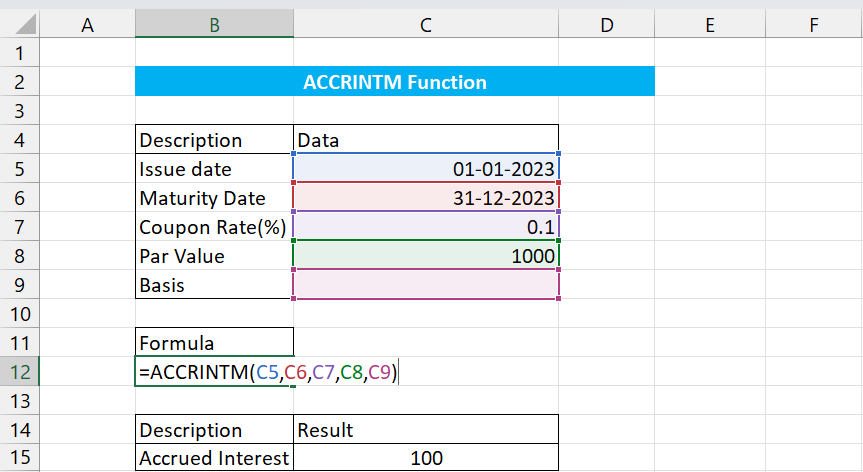
In this picture, one can see the Accrued Interest payable in Cell B12 using the ACCRINTM formula.
Example 3: Number as dates & Referencing.
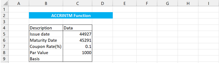
Here, we can see that we have neither used the date formatting in the cells nor the DATE Function but rather used random numbers.
Well, these numbers aren't exactly random. In Excel, dates have serial numbers; here, 45291 represents 31st December 2023, and 44927 represents 1st January 2023.
This function of Excel isn't very widely used and not very preferable too.
However, we will look at this example using these numbers as dates.
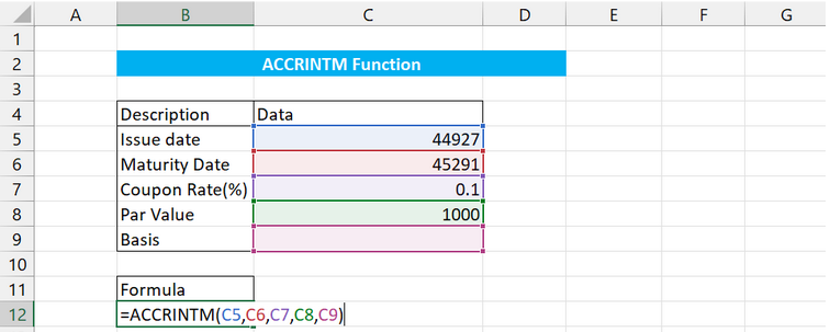
Here, we have referenced C5, C6, C7, C8, and C9 according to the syntax of the ACCRINTM Function, as discussed earlier.
Example 4: DATE Function & Hardcoding
Unlike the examples where we have used Cell Referencing, we will be hardcoding the arguments.
Suppose you are asked to find out the accrued interest on a bond issued on 1st January 2023 with a coupon rate of 5% and FV of 100, and the settlement date being the End of Next Year, i.e., 31st December 2024.
We will skip the [basis] part since there is no information.
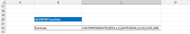
We will use the it shown in Cell C22 above.
We use the DATE Function to avoid any mistakes occurring due to different interpretations of dates and the complexity of using numbers as dates.
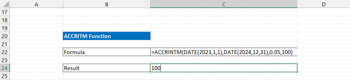
Using the function, we arrive at a result shown in Cell C24.
By looking at the four examples above, one can understand how the ACCRINTM Function is used in MS Excel.
ACCRINTM Function: Points to remember
There can be other problems that might occur while using this function. Here are some points you must remember while using this function since it can help you to use it more easily and productively.

1. The calculation for the ACCRINTM function is as follows:
ACCRINTM = Par * Rate * A/D
Where,
- A: Accrued days are counted on a monthly basis. When it comes to items involving interest on maturity, the number of days between the issue and settlement date are considered.
- D: Day count basis/ Annual year basis.
2. Dates are stored in MS Excel in sequential serial numbers so that they can be used in calculations.
1st January 1900 is Number 1 by default, and so on; for example, Number 15 will give the date of 15th January 1900 since it is 15 days after 1st January 1900. Similarly, other dates can be found.
3. The #NUM! error will be returned if the rate is 0 or negative or if the par value is 0 or negative, as interest rates and par values cannot be negative.
=ACCRINTM(“1/1/2022”,”1/1/2023”,-1,,7) will return #NUM
=ACCRINTM(“1/1/2022”,”1/1/2023”,1,-1000,7) will return #NUM
4. The return value will be #NUM! Error if the basis is lesser than 0 or more than 4 since only either of these 5 values (or omission) are allowed, as discussed in the table above.
=ACCRINTM(“1/1/2022”,”1/1/2023”,1,,7) will return #NUM!
5. The return value will be #NUM! Error if the issue date is greater (meaning after) than the maturity date since the maturity cannot be before the issue of security.
=ACCRINTM(“1/1/2023”,”1/1/2022”,0.5,,1) will return #NUM!
6. The return value will be #VALUE! Error if the issue date or settlement (maturity) date is not valid.
=ACCRINTM(“WSO”,”1/1/2022”,0.5,,1) will return #VALUE!
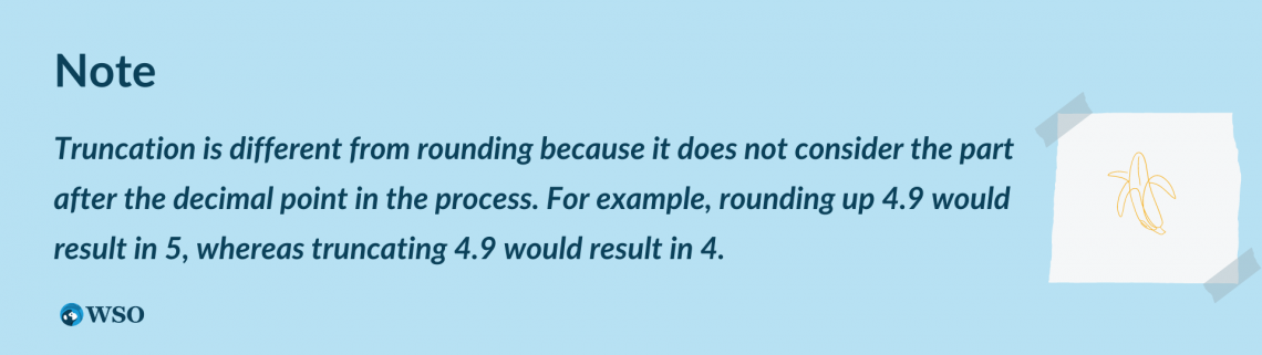
7. If the Issue date (issue), settlement date(settlement), and basis are in decimals, then they would be truncated into integers. The arguments can be referenced to other cells, hard-coded, or a mix of both.
8. To avoid misinterpretation of dates due to different settings and data interpretation techniques in Excel, it is recommended to use the DATE function.
9. Ensure the day count basis used is the proper one since it can make a difference in the final interest accrued.
10. Ensure that dates are in a consistent format or are used using the DATE function in Excel; also, the rate must be in percentage, i.e., 5% will be 0.05 in the formula if it is hard coded.

Free Resources
To continue learning and advancing your career, check out these additional helpful WSO resources:


or Want to Sign up with your social account?