CEILING.MATH Function
A Mathematics &Trignometry function in Excel that rounds a number up to the nearest integer or to a specified multiple in the spreadsheet.


What is the CEILING.MATH Function?
The CEILING.MATH function is a Mathematics &Trignometry function in Excel that rounds a number up to the nearest integer or to a specified multiple in the spreadsheet.

If there’s something Excel can do really well, it is number operations, whether simple operations such as addition or subtraction or more complex formulas.
One of those is also rounding up numbers away from zero or towards zero.
Generally, Excel follows the rounding principle wherein the value rounds toward zero if the number falls between zero and four. If the number falls between five and nine, it rounds away from zero.
Where does the CEILING.MATH function comes into all these scenarios.
Well, it is one of the functions that have the capability to round up a number, but of course, there’s a catch. So let’s see what is the CEILING.MATH function, how to use it, and a couple of examples.
- The CEILING.MATH function is categorized as a Math & Trigonometric function that rounds a number to a specified multiple.
- The CEILING.MATH function accepts three arguments: number, significant, and mode, the latter two of which are optional.
- The function is commonly used in data formatting to round numbers up to more user-friendly or standardized values, improving the clarity and readability of reports and presentations.
- CEILING.MATH function finds applications in fields such as finance, engineering, and data analysis, wherever precise rounding up of numbers is required to achieve desired outcomes.
How CEILING.MATH function works
The CEILING.MATH is a categorized Math and Trigonometric function that rounds up a given number to a specific multiple.
For example, if the number is 1.456 and needs to be rounded to the multiple of 2, then the obvious answer is 2. However, if the number were rounded to the multiple of 13, the result would have been 13.
Similarly, if the number were 47.9, the number rounded to the multiple of 2 would be 48. Again, the same number rounded to the multiple of 3 would give the result of 51.
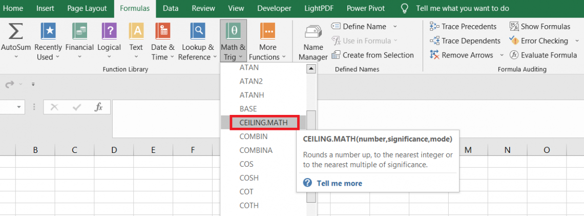
The syntax for the CEILING.MATH function is:
=CEILING.MATH(number, [significance],[mode])
Where,
- number - (required) the value which will be rounded off
- significance - (optional) the multiple up to which the given number will be rounded. If the argument is skipped, the function assumes the default value of 1.
- mode - (optional) reverses the direction of rounding exclusively for negative numbers. The argument accepts two values - zero to round the negative numbers toward zero and any other numerical value to round negative numbers away from zero.
Example for the CEILING.MATH function
In the previously written episode of the CEILING.MATH function, we saw what the syntax was. Nothing special, just a couple of arguments, amongst which two were optional. Still, they hold crucial importance if you bring out the function's full potential.
Suppose you have some of the numbers in Excel as illustrated below:
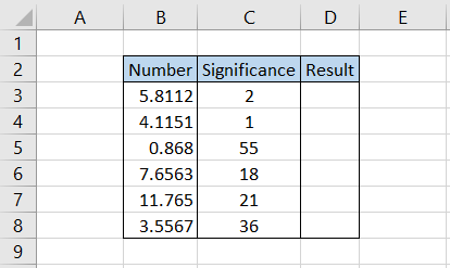
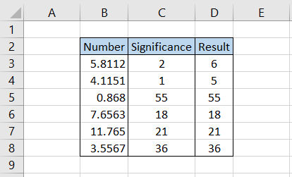
To find the rounded number based on specified multiples, we will use the formula =CEILING.MATH(B3,C3) in cell D3 and drag it down till cell D8, which gives the result:
Interpretation:
- In cell B3, we have the number 5.8112, and the multiple mentioned is 2. Now, the multiples of the number 2 are 2,4,6,8, and so on. Since the nearest multiple to the number is 6, we get the same result in cell D3.
- In cells B4 and C4, we have values of 4.1151 and 1, respectively. The multiples of 1 are 1,2,3,4,5...so on. Thus, the function rounds up the number to 5.
- The numbers in range B5:B8 are evaluated on a similar basis, and their rounded-up numbers are returned in range D5:D8.
Mode Argument in the CEILING.MATH Function
We saw what the significance argument does in the CEILING.MATH function, and honestly, it does hold a lot of ‘significance.’ But what even is the mode argument?

If you are a mathematical geek, then you must be aware that mode is the number that makes the most appearances in a given dataset. Excel even offers a function to find that particular number using the MODE function.
But this is not the same mode we are talking about.
You see, this argument specifically works for negative numbers. The argument will accept only two values - either zero or any other number.
If you input zero, the negative number will be rounded toward zero. If any other number is input, the function rounds away from zero.
First, let’s see how the ‘mode’ argument actually works. Suppose you have the data as illustrated below:
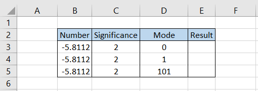
Here, we have the same number and the significance value, but the only difference is in the value of the mode. We will use the formula =CEILING.MATH(B3,C3,D3) in cell E3 and drag it down till cell E5, which gives the result:
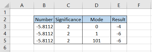
As you see, when the value of mode is equal to zero, the number gets rounded toward zero irrespective of the original number. In contrast, when the value is anything other than zero, the number gets rounded away from zero.
How would the results differ if we compare the positive and negative numbers? For example, suppose the data looks as illustrated below:
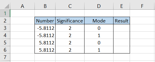
We have the same number represented as positive and negative, along with different values for mode. After using the formula =CEILING.MATH(B3,C3,D3) in cell E3 and dragging it down till E6, we get

Either way, the positive numbers are unaffected by the value in the mode argument. However, it's an entirely different story when the argument is used for negative numbers, as represented in the example above for the CEILING.MATH function.
Practical Example of the CEILING.MATH function
How would you use the CEILING.MATH function in real life?
Let’s see a really simple example of how you can use the function to determine the number of stocks you can purchase for your portfolio.
Suppose Microsoft Corp is trading at $286.14 on NASDAQ. You have a disposable amount of $2500, which can be invested in the stock. How many stocks can you buy with the current corpus?
The data looks as illustrated below:
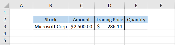
After using the formula =CEILING.MATH(C3,D3)/D3-1 in cell E3, we get the result:
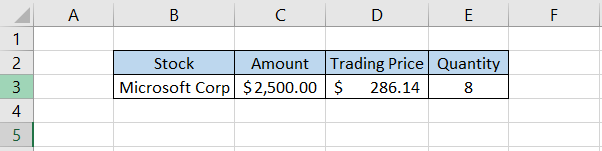
Let’s break down the formula a bit. First, we will just use simple CEILING.MATH formula gives the result as $2575.26. Next, we divide this value by the trading price of the stock, which gives the result of 9.
This means that Excel wants to say that you can buy 9 quantities of stock with the amount. But this is not the true answer. First, remember that Excel is evaluating the quantity based on the amount of $2575.26 and not $2500.
Thus, we will subtract 1 from the result, giving the quantity 8.
Subtracting one from the result gives the actual value for quantity since we do not have an additional disposable amount for purchasing the stocks.

Other Rounding functions
There are several functions that round the number or remove the decimal digits from a given number, such as ROUND, ROUNDUP, ROUNDDOWN, TRUNC, etc.

Each function is unique since they work on the unique principle they are built upon.
Although we have covered each of these functions separately, we will try to understand how these functions differ from CEILING.MATH.
a. ROUND
The ROUND function works on the rounding principle wherein when the ‘nth’ digit lies between zero and four, the number gets rounded down, while if the ‘nth’ digit is between five and nine, the number gets rounded up.
Suppose we have the data as illustrated below:
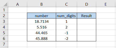
By using the formula =ROUND(B3,C3) in cell D3 and dragging it down till cell D6, we get
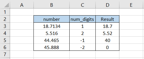
When you round the number 18.7134 to the first digit after the decimal, we get the result as 18.7. Since the second digit lie between zero and four, the number rounds down toward zero.
Similarly, when the number is 5.516 and needs to be rounded to the second digit, we see that the third digit lies between five and nine. As a result, the number gets rounded up away from zero.
A similar trend follows for the rest of the numbers in the example. When a negative value is used for the num_digits argument, the digits before the decimal are rounded but based on the same principle.
b. ROUNDUP
ROUNDUP will round a number away from zero, and the additional condition is that this happens despite what the ‘nth’ digit is.
So whether the ‘nth’ digit after the decimal is 2 or 9, the function will always round the number up away from zero.
Suppose we have the data as illustrated below:
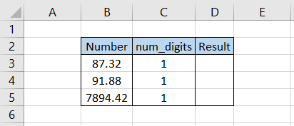
After using the formula =ROUNDUP(B3,C3) in cell D3 and dragging it down till cell D5, we get
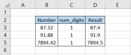
You see, we wanted to round the number to the first digit after the decimal point. Of course, the second digit after decimal has been 2 and 8, but the number always got rounded up away from zero.
c. ROUNDDOWN
ROUNDDOWN works precisely opposite to that ROUNDUP. The function will always round towards zero, regardless of the ‘nth’ value.
For example, suppose we have the data as illustrated below:
The results are now completely contradictory. The numbers that were rounded up before get rounded down toward zero. By using the formula =ROUNDDOWN(B3,C3) in cell D3 and dragging it down till cell D5 we get
Do you see why we said each function works on a unique principle? So each can be used in a different scenario to return a result as per the conditions we are working under.
d. TRUNC
TRUNC is a far more special function. The function holds the ability to remove the unwanted digits after the decimal point with just a couple of arguments.
The number doesn’t get rounded, but the function cancels out the digits after the decimal.
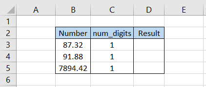
For example, suppose we have the data as illustrated below:
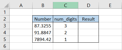
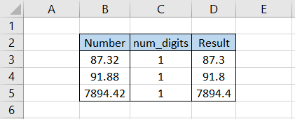
By using the formula =TRUNC(B3,C3) we get the result as:
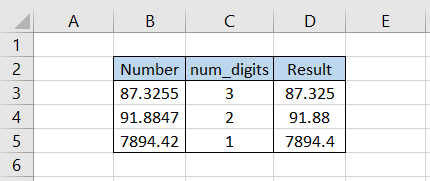
As you can see, as per our instructions to limit the digits after the decimal to three, two, and one, respectively, the function returns the result in column D.

Free Resources
To continue learning and advancing your career, check out these additional helpful WSO resources:


or Want to Sign up with your social account?