CHISQ.DIST.RT Function
One of the Statistical Functions in Excel that calculates the right-tailed probability of the chi-squared distribution.


What is the CHISQ.DIST.RT Function?
The CHISQ.DIST.RT Function in Excel is one of the Statistical Functions that calculates the right-tailed probability of the chi-squared distribution. CHISQ.DIST.RT Function is utilized to test the Chi-Squared test to compare observed values with expected values.

This distribution can only be used for chi-square (χ2) distributions, which occurs when comparing sample outcomes to each other or the population/expected results.
German statistician Friedrich Robert Helmert first discovered this distribution in 1876. Karl Pearson, known as the father of statistics, later explored the distribution through the goodness of fit, one of the three main uses of a χ2 test.
Chi-square distributions are used across various disciplines. For example, scientists would use this to determine if there are side effects from mixing two specific medications, as the scientist would be testing for the independence of the drugs.
This distribution has implications for businesses when conducting fieldwork to analyze the tastes of (potential) customers. Market research is not very helpful unless you know how to interpret the collected data properly!
-
The CHISQ.DIST.RT function is an Excel Statistical Function used to calculate the right-tailed probability of the chi-square distribution.
-
The CHISQ.DIST.RT function calculates the probability that a value from a chi-square distribution with given degrees of freedom is less than or equal to a specified value.
-
The CHISQ.DIST.RT function typically doesn't encounter errors unless the provided arguments are non-numeric or out of range. In such cases, it may return an error value.
-
The CHISQ.DIST.RT function returns the right-tailed probability of the chi-square distribution, which represents the probability of observing a value less than or equal to the specified value.
Chi-Squared Tests Explained
Chi-squared tests are used to compare categories in a sample with others or the population. This is different from p-tests and t-tests as those compare one outcome in a sample to the population.

There are three types of chi-squared tests:
- The test of goodness of fit
- The test of independence
- The test for homogeneity
The goodness of fit test compares the distribution of items of categorized groups in a sample to their proportions in the population or compares the observed and expected categorical proportions.
The test of independence compares two samples of the same population to determine if the groups within the sample are independent of each other. The test for homogeneity is executed the same as the test of independence but compares samples of different populations.
NOTE
All three tests: the test of goodness of fit, the test of independence, and the test for homogeneity, can be conducted using Excel’s chi-squared right-tailed function.
To understand how this is carried out in Excel, it is essential to comprehend the math behind it. However, before we dive into specifics on each, we need to discuss the aspects that are the same between the three.
When beginning any problem, two hypotheses must be made;
- the null hypothesis (HO) and
- the alternative hypothesis (Ha).
The HO predicts no correlation between the groups being compared in the test, whereas the Ha predicts a correlation between the groups.
Another similarity is the use of an alpha (𝛼) value. This is the maximum percentage of difference for the data to be statistically significant. If not specified, it can be assumed that the 𝛼 value is 5%.
Interestingly, 95% is the typical statistician’s confidence level, meaning they are 95% confident that something will occur, whether in a statistical test or when constructing a confidence interval. This indicates there is a 5% chance that something will happen otherwise.
For the alternative hypothesis to be accurate, the percentage we get when we run the test must be lower than the 𝛼 value. This can be seen easily in the graphical representation of a chi-squared distribution graph.
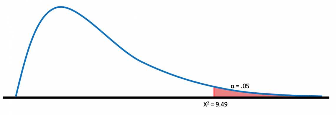
This graph shows the alpha value in the area within 5% of the right tail. If the χ2 we calculate is less than the alpha value, it will fall under the shaded range, and there is a statistically significant correlation.
However, suppose we calculate a χ2 greater than 5%. In that case, it will fall before the shaded region, and there will not be statistically significant evidence to indicate a correlation between the compared groups.
It is important to note that not every chi-squared distribution has a graph like the one above. It depends on the degrees of freedom (k) based on the sampling size (n). It can be estimated by subtracting one from the sample size; the formula for this is:
k = n - 1
In the graph below, we can see just how drastically the chi-squared distribution changes with degrees of freedom:

Thus, degrees of freedom are significant, as a slight error could significantly change the output by inputting the degrees of freedom, Excel processes which distribution it needs to use.
CHISQ.DIST.RT Function Explained
Excel has created a function to give users a way to calculate the right tail probability of a χ2 test without using data.

The formula for conducting a right-tailed chi-squared test is
=CHISQ.DIST.RT(x,deg_freedom)
Where
- x (required) is the left bound for the area you are calculating the probability for
- deg_freedom (required) is the degree of freedom.
By asking for minimal inputs, this function can significantly help calculate a probability in a scenario you do not know much about. In statistics, one small change to a trial’s value can greatly affect the final result, and this function makes this problem obsolete.
An example where this could come in handy is when you know the sample size is 10 and you are looking for a right-tailed probability of 7.9.
Using the sample size, we can calculate the degrees of freedom:
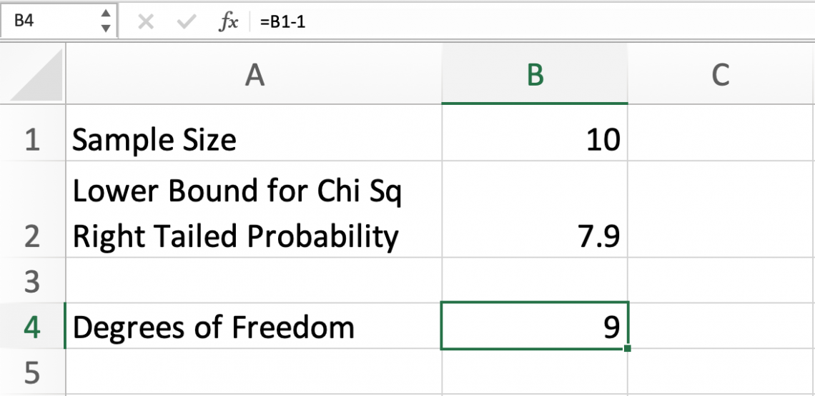
All χ2 scenarios with the same degree of freedom have the same distribution. Excel needs this argument to understand which type of distribution it is referencing.
Now we have both arguments of the function; we can calculate the right tail probability:
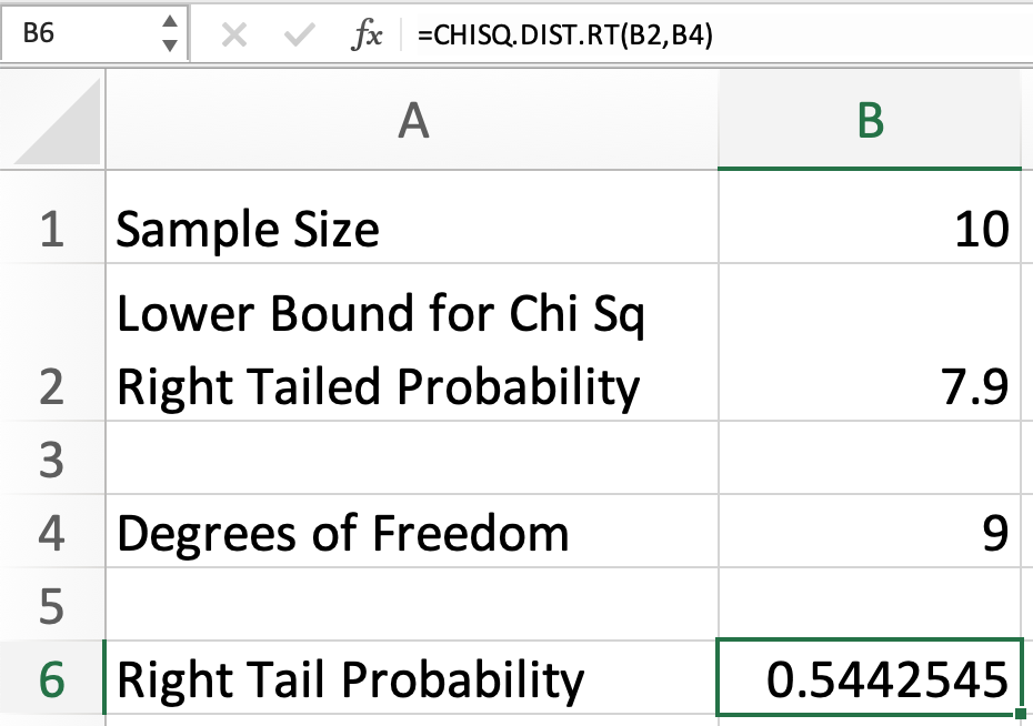
This indicates that in a distribution where the degree of freedom is 9, the right tail probability for 7.9 is .5443, or 54.43%.
Now that we understand how to use the function, we can look at a more in-depth χ2 test and how the CHISQ.DIST.RIGHT function can fit in.
Example: Goodness of Fit Test
In this example, we will conduct a goodness of fit test to compare the observed and categorical proportions of expected and observed values of blue jelly beans in different bags of the same brand.
| Jelly Beans | Bag 01 | Bag 02 | Bag 03 | Bag 04 | Bag 05 |
|---|---|---|---|---|---|
| Expected | 5 | 7 | 8 | 4 | 9 |
| Observed | 6 | 9 | 9 | 7 | 8 |
Our first step is to write out our null and alternative hypotheses:
- HO: There is no difference in frequency in the data
- Ha: There is a difference in frequency in the data
Next, we need to define our 𝛼 value. Because this was not described in the problem, we can assume it is 5%, or 0.05.
Next, we need to find our degrees of freedom, which can be calculated using the following formula:
k = n - 1
k = 5 - 1
k = 4
NOTE
Be sure to note that the sample size is 5, as there were 5 observed instances, not 10.
Next, we need to locate the value in the following table that corresponds with an 𝛼 value of .05 and k of 4.
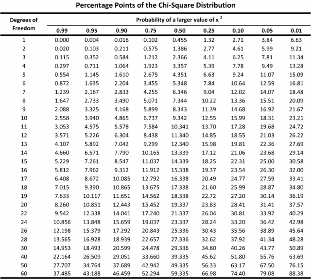
This is called the critical value, which is 9.49. This means that for the data to have a statistically significant difference, the χ2 value must be at least 9.49.
Now, we need to calculate the χ2 value for the situation. For the goodness of fit test, this can be done using the following formula:

Our calculated χ2 test of 3.26 is less than the critical value of 9.49, meaning we accept our HO. Therefore, we found no significant difference between the expected and observed values.
This can be paired with the Excel formula, which will find the probability of the value lying to the right of the χ2 test answer, which is 3.26.
As a refresher, the Excel formula is
=CHISQ.DIST.RT(x,deg_freedom)
Now, we can fill in the arguments for the formula:
- x: 3.26 (our calculated chi-squared value)
- deg_freedom: 4 (this was calculated using k=n-1)
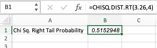
This test shows a .5153, or 51.53%, chance of no difference in the data.
In this example, the χ2 test might feel unnecessary, as we could have referenced the table from earlier to determine the right tail probability using the x value and degrees of freedom. In this case, a different formula might be a better fit.
CHISQ.TEST Excel Function
CHISQ.TEST is often a more helpful tool than CHISQ.DIST.RT, as the former, can do the entire chi-squared test.

The arguments for the function are seen below
=CHISQ.TEST(actual_range,expected_range)
Where
- actual_range (required) includes the observed values in the sample.
- expected_range (required) includes the sample values anticipated to occur.
We can type our data into an Excel sheet and use this function to conduct the χ2 test. But first, we should establish what each argument will be:
- actual_range: Cell names of the “Observed” row
- expected_range: Cell names of the “Expected” row
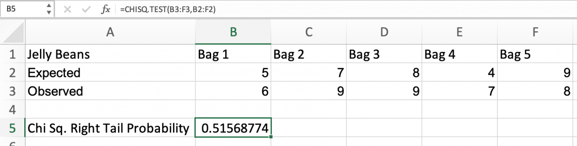
Because this test's result (51.57%) is higher than the 𝛼 value, we can conclude that there is no statistically significant evidence of a difference in the data.
This was an extremely efficient way to solve a full χ2 test. You may be wondering why the probability when calculating using CHISQ.DIST.RT vs.CHISQ.TEST happens for two reasons: degrees of freedom and rounding our values.
The degrees of freedom formula we used when doing the test by hand (subtracting 1 from the sample size) is not an exact value but a close estimate. When a computational device calculates the degrees of freedom, it often uses a complex formula.
Additionally, when we entered values for CHISQ.DIST.RT, they were rounded. The 3.26 figure has many decimal places, so the value entered into Excel was rounded. Our results would be much closer if we entered the 3.26 figure with all its decimals.

Free Resources
To continue learning and advancing your career, check out these additional helpful WSO resources:


or Want to Sign up with your social account?