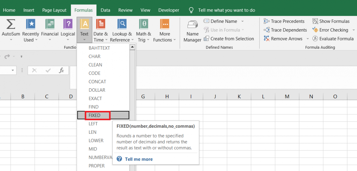
FIXED Function

What is the FIXED Function?

The fixed function in Excel returns a number rounded to a specified number of decimal places as a text representation.

The function here has two core components: rounding a number to ‘n’ decimal places and another is to represent the result in the form of the text value.

We have already seen a lot of rounding functions, such as ROUND, ROUNDUP, ROUNDDOWN, etc., which can ‘round’ a numerical value based on the rounding principle.

In general, the rounding principle means when the ‘nth’ digit lies between zero to four, the number gets rounded down, whereas if the ‘nth’ digit lies between five and nine, the number gets rounded up.

However, one major difference distinguishes the FIXED function and other rounding functions.

Let’s see the FIXED function and understand those differentiating factors by how the function works.

Understanding the FIXED function

The FIXED is categorized as a Text function that rounds a number to a specified number of decimal places and then represents it as text.

Rounding off a number happens when a given digit gets rounded up or down. For example, 34.89 rounded to the first decimal digit becomes 34.9. The FIXED function works on a similar principle and returns the rounded number to the user.

Another example of this rounding phenomenon is when the revenue earned for FY by a company such as Nvidia Inc is $26.914B, and the FIXED function gives the result as $26.9B. But again, this number is rounded down to its first decimal digit.

However, the major factor differentiating other rounding functions and FIXED is the latter’s ability to return the rounded value as a text string.

FIXED Function Formula

How do we even verify this particular statement? It is possible to determine this with the help of a particular function already in Excel. But first, let’s head over to the syntax for the function:

where,

• number - (required) the numerical value which will be represented as the text string
• decimals - (optional) the number of decimal digits up to which the given number will be rounded off.
  • If the argument is ignored, the function assumes a default value of 2, whereas a negative integer rounds the number to the left of the decimal point.
• no_commas - (optional) specifies whether numerical values returned as text be separated by commas(i.e., thousands, millions, etc.).
  • The argument can accept two values: TRUE, where commas are not included in the text, and FALSE, where text is included.
  • If the argument is ignored, then the function assumes the default value of FALSE.

How to use the FIXED Function in Excel?

Let’s jump onto an example to understand how the function works. We will even see how to identify if the numerical has been changed into the ‘text’ datatype or if it is still a number.

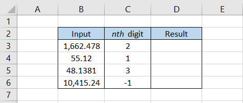
Suppose you have the data as illustrated below:

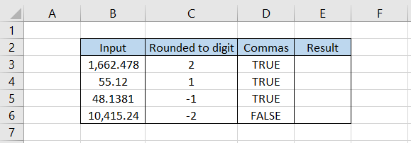
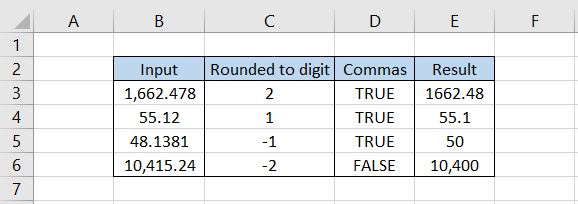
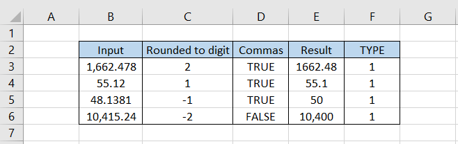
After using the formula =FIXED(B3,C3,D3) in cell E3 and dragging it down till cell E6, we get

Interpretation:

• In cell B3, we have the number 1,662.478, rounded to two digits after the decimal giving the result as 1662.48. Since we have used the optional argument for no_commas as TRUE, it eliminates all the commas from the number.
• The number 55.12 has ‘1’ in its first digit after the decimal. As it lies between zero and four, the number gets rounded down and returns 55.1. Initially, the number did not have commas, so there is no effect of the no_comma argument.
• In cell B5, the number 48.1381, rounded to a negative one, gives the result as 50. This time, we are looking for the digit before the eight decimals. Since it lies between five and nine, the number gets rounded up to 50.
• Finally, the number 10,415.24 is separated by commas, and it is to be rounded to two digits before the decimal. In such a case, the result is 10,400 since the second digit before the decimal is one. 

Also, the comma gets retained since we used the no_commas argument as FALSE.

Identifying the data type of the result

Now, the only thing that needs to be answered is how to identify whether the returned result is a number or a text value.

We will use the TYPE function to verify whether the referenced value is a text string or a number. The TYPE function returns an integer value for different data types in Excel.

For example, if you reference a number, the function returns the result as 1, whereas if a text string is referenced, the function returns the result as 2.

Thus, when you use the formula =TYPE(E3) in cell F3 and drag it down to cell F6, we get the result:

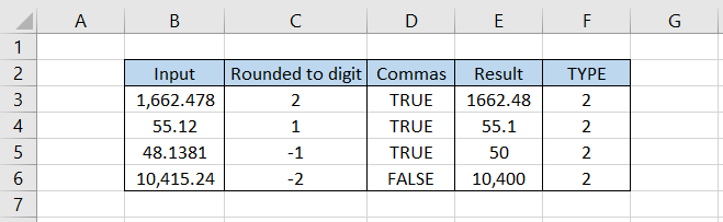
All the numbers in column E are stored as text strings and not as numbers. In contrast, when you reference the values in column B using the formula =TYPE(B3) in cell F3 and drag it to cell F6, then the result is

This confirms that values in column B are numbers, whereas column E values are text strings.

You can use the VALUE function to revert the number represented as text strings to its factory setting.

We won’t go into depth about how the function works, but you only need to use the formula =VALUE(E3) in cell F3 and drag it down until cell F6. Then, later on, you can use the =TYPE(F3) formula in cell G3 and drag it down to cell G6, which gives the data type as 1.

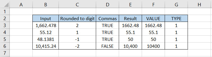
This means the referenced cell value is a number, not a text string.

Alternatives to the FIXED function

Based on the functionality of rounding the numbers, you can use a few alternatives in Excel apart from the FIXED function.

You might already know some of these, such as ROUND, ROUNDUP, ROUNDDOWN, etc. Another function that does not round a number but rather just limits a number to the ‘nth’ decimal digit is the TRUNC function.

In this section, we will see all these alternatives and an example.

a. ROUND function

Based on the rounding principle, the ROUND function will round a given numerical value. If the ‘nth’ digit number lies between zero and four, then the number gets rounded down; if the number lies between five and nine, then the number gets rounded up.

The syntax for the function is

=ROUND(number, num_digits)

where,

• number - (required) the numerical value which needs to be rounded off
• num_digits - (required) the ‘nth’ place before or after the decimal up to which the number will be rounded off.

Suppose you have the data as illustrated below:

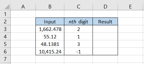
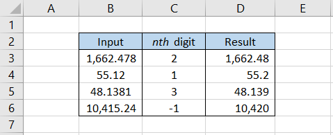
By using the formula =ROUND(B3,C3) in cell D3 and dragging it down to cell D6, we get

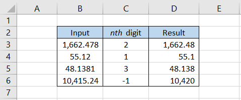
The numbers in column B get rounded off according to the founding principle. ROUND is the most popular rounding function amongst Excel users due to its simplicity and accuracy with which it returns the result.

b. ROUNDUP function

The next two functions are quite peculiar, but first, let’s focus on ROUNDUP. The ROUNDUP function does not follow the rounding principle and will always round up a number irrespective of the digit at the ‘nth’ position.

The syntax for the function is

=ROUNDUP(number, num_digits)

where,

• number - (required) the number which will be rounded up
• num_digits - (required) the ‘nth’ place up to which a number will be rounded up.

Suppose we have the data as illustrated below:

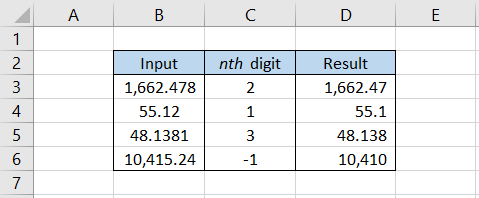
By using the formula =ROUNDUP(B3,C3) in cell D3 and dragging it down to cell D6, we get

As you can see, even though the function still rounds up the value when we had a number between zero and four at the ‘nth’ place before or after the decimal. The general rounding principle does not apply to the ROUNDUP function.

c. ROUNDDOWN function

The ROUNDDOWN function works opposite to that of the ROUNDUP function. Again, it does not work according to the rounding principle but always rounds down a value irrespective of the number at the ‘nth’ place.

The syntax for the function is

=ROUNDDOWN(number, num_digits)

where,

• number - (required) the number which will be rounded down
• num_digits - (required) the ‘nth’ place upto which a number will be rounded down

Suppose you have the data as illustrated below:

By using the formula =ROUNDDOWN(B3,C3) in cell D3 and dragging it down to cell D6, we get

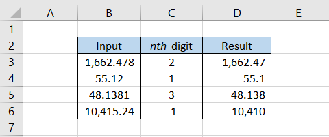
In this case, irrespective of the number at the ‘nth’ place, the number gets rounded down away from zero.

The function does not follow the rounding principle evident from the result 1662.47, where despite the number 7 falling between five and nine, the number rounds towards zero.

d. TRUNC function

The TRUNC function does not round a number but truncates a number to the ‘nth’ decimal place. When we talk about truncating a number, it means limiting a number to that particular digit after the decimal.

Thus, a number 36.8265 limited to two decimal digits will give the result as 36.82. Here, the rounding principle does not apply to return the numbers to the user.

The syntax for the function is

=TRUNC(number, [num_digits])

where,

• number - (required) the number which will be truncated
• num_digits - (required) the ‘nth’ digit upto which the number will be truncated

Suppose we have the data as illustrated below:

By using the formula =TRUNC(B3,C3) in cell D3 and dragging it down till cell D6, we get

It is quite evident from the result that no particular rounding phenomenon takes place. The function limits the decimal digits to the ‘nth’ decimal place.

Free Resources

To continue learning and advancing your career, check out these additional helpful WSO resources:

• DOLLARDE Function
• DOLLARFR Function
• NUMBERVALUE Function
• PRICE Function
• PRICEMAT Function