INTRATE Function
One of the Excel Financial Functions that calculates the interest rate for a ‘fully invested’ security redeemed at maturity.


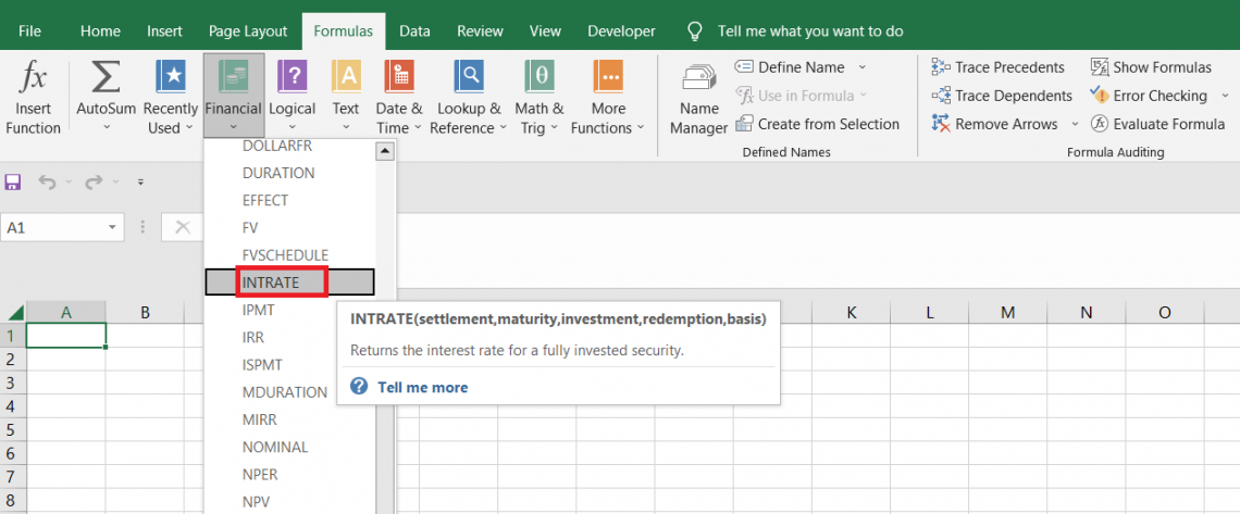
What is the INTRATE Function?
The INTRATE function is one of the Excel Financial Functions that calculates the interest rate for a ‘fully invested’ security redeemed at maturity.
Unlike other securities, a fully invested alternative does not pay periodic interest before maturity. A zero coupon bond could be one example of a fully supported bond in which the investor receives the interest income only after the security redemption.
The interest income is the difference between the price at which the bond was purchased and the price at which the bond will be redeemed after maturity.
Thus, the function becomes an effective tool for calculating the interest rates for such investable securities.
In this article, we will learn how to use the INTRATE function and use a couple of examples to help us understand it better.
- The INTRATE function is part of Excel Financial Functions and calculates the interest rate for a fully invested security.
- Users provide arguments, including the settlement date, maturity date, investment, redemption value, and basis. It returns the annual interest rate for the investment.
- Users might encounter potential errors when using the INTRATE function, such as providing invalid dates, referencing cells with incorrect data, and not knowing how to address them effectively.
- The INTRATE function aids in financial analysis by providing insights into an investment's effective interest rate, allowing investors to assess the profitability and attractiveness of investing in such securities.
Understanding The INTRATE function
INTRATE is a Financial function that calculates the interest rate for a security in which the investor is fully invested.
For example, suppose an investor buys a bond for $90 on 1 January 2023 and sells it for $99.30 at maturity on 30 March 2026.
During this period, the person does not receive any interest component, which is ultimately received at the time of maturity along with the principal part.
The annualized interest rate for the said security can be calculated using the INTRATE function in Excel, which equals 3.18%.
INTRATE function Formula
The syntax for the function is
=INTRATE(settlement, maturity, investment, redemption, [basis])

where
- Settlement - (required) the settlement date for the security (usually two days after the purchase of a security)
- Maturity - (required) the date on which the security matures and the invested amount is returned to the investor
- Investment - (required) the amount that is invested in the said security
- Redemption - (required) the amount that is returned to the investors upon the maturity
- Basis - (optional) The day-counting basis that will be used for the fully invested security
It can take different values, as illustrated below:
| Basis Value | Day Count Basis |
|---|---|
| 0 / default | US (NASD) 30/360 |
| 1 | Actual/actual |
| 2 | Actual / 360 |
| 3 | Actual / 365 |
| 4 | European 30/360 |

How to use the INTRATE Function in Excel?
You need to consider four essential arguments before using the function. The function will return an error if you miss either of those arguments.
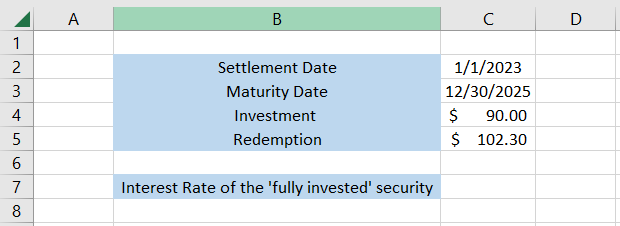
Suppose you have the data in Excel as illustrated below:
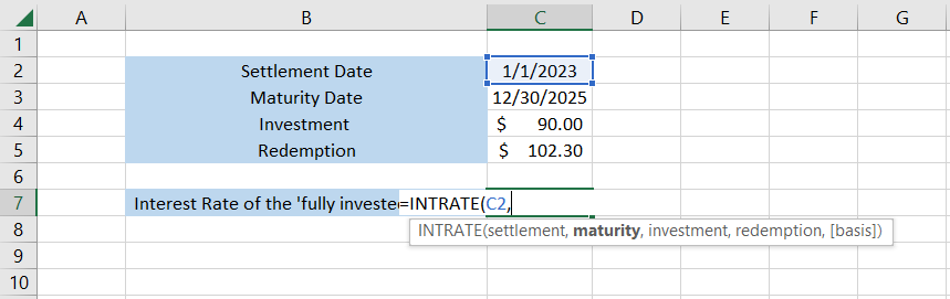
1. Settlement
The settlement argument refers to the settlement date of the said security. When you purchase the protection from the market, it usually gets settled into your account on T+2 day.
For example, if the security is purchased on 29th December 2022, it gets settled on 1st January 2023.
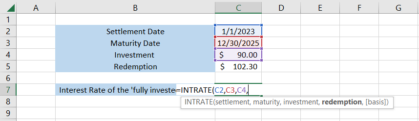
In this example, the settlement date is in cell C2, so the formula in cell C7 becomes =INTRATE(C2, maturity, investment, redemption, basis) as below:
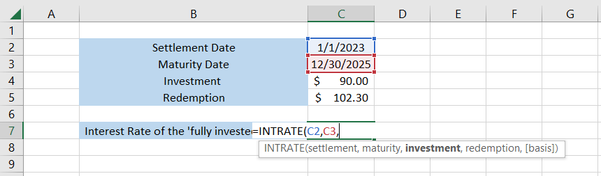
2. Maturity
It is the maturity date of the security. This is when the deposit's holding tenure ends, and the invested amount is returned to the investors.
The maturity date for the said security is given in cell C3. The formula in cell C7 becomes =INTRATE(C2, C3, investment, redemption, basis)
3. Investment
The invested amount in the security is the third important argument that the function needs to calculate the interest rate for a fully funded financial product. The invested amount is $90, which is in cell C4.
The formula becomes =INTRATE(C2, C3, C4, redemption, basis) as below
4. Redemption
The amount redeemed to the investor at the end of the maturity period is the fourth argument in the function.
The redeemed amount is the combination of the invested principal amount and the accrued income, usually not paid to the investor as a coupon payment.
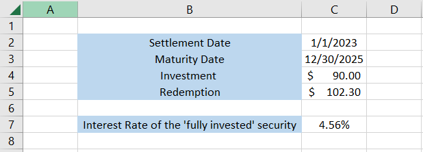
The formula becomes =INTRATE(C2, C3, C4, C5, basis), giving the result in cell C7 as 4.56%.
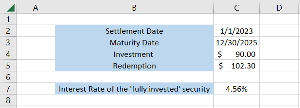
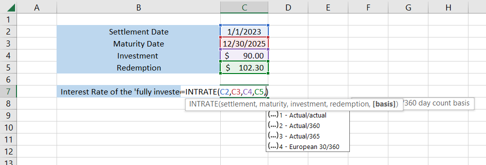
This is the interest rate for the fully invested security. You must wonder why we haven’t included the basis argument in the formula.
By default, the function uses the argument as zero, meaning Excel uses the US (NASD) 30/360 convention to calculate the interest rate.
However, you can select any other acceptable value, and the function automatically transforms the final result depending on what day convention you use in the role.
5. Basis
To understand whether there is any difference in the result, let’s choose some other ‘acceptable’ value for the basic argument.
Suppose we select the argument as 3, which selects the Actual/365-day convention. Then, the formula becomes =INTRATE(C2,C3,C4,C5,3), which gives the result:
Even though we don't see any significant difference, the only changes that happened were beyond the sixth or seventh decimal number. You can use different day conventions to return the result as required.
INTRATE Function Example
Let’s see a couple of examples to understand further where you can best use the function.
Example 1
Suppose you purchase a zero coupon bond at $95.23 with a settlement date of 17th January 2023. The bond finally matures on 31st January 2024 at $101.23.
The data looks as illustrated below:
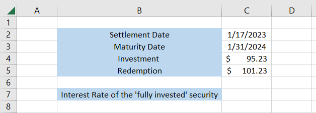
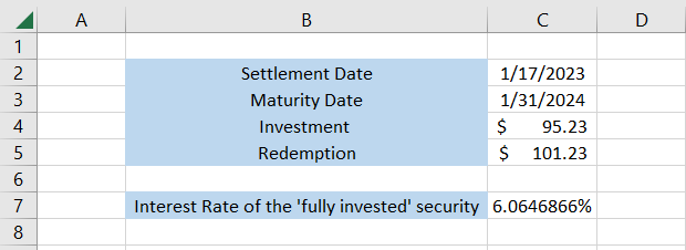
To calculate the annualized interest rates, we will use the formula =INTRATE(C2,C3,C4,C5,0), giving the result 6.04% for the ‘fully invested’ security.
Thus, the INTRATE function makes it easier to calculate the interest rate for the security.
Example 2
The function allows you to compare two fully invested securities to understand which had the higher interest rate.
Suppose you have the data as illustrated below:
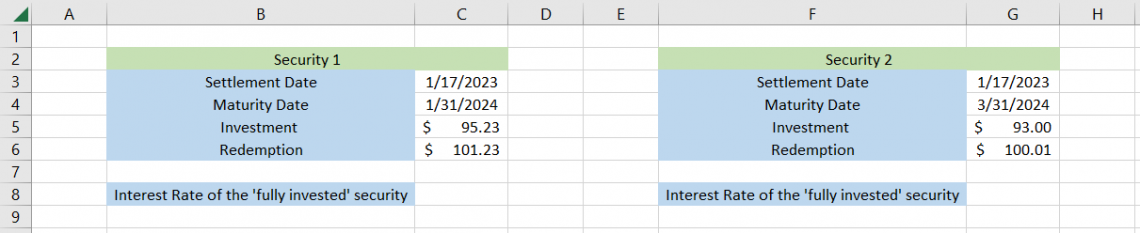
The only data we have similar to the example below is the settlement date equal to 17th January 2023.
To calculate the interest rate, we will use the formula =INTRATE(C3,C4,C5,C6,0) in cell C8 and =INTRATE(G3,G4,G5,G6,0) in cell G8, which gives the result:
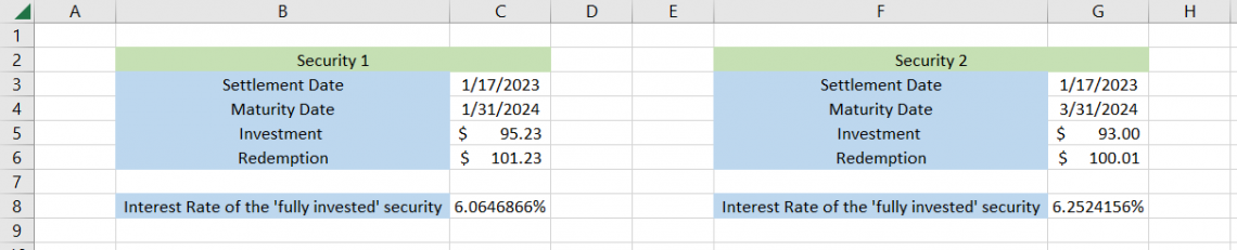
Thus, we can interpret that all three arguments, maturity, investment, and redemption, function independently, causing the interest rate to fluctuate accordingly in the final result.
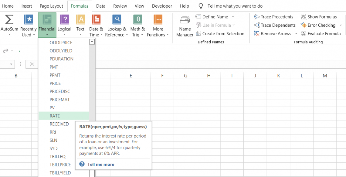
INTRATE vs. RATE function
In terms of functionality, the RATE function comes closest to what INTRATE can do. The RATE is a financial function that calculates the interest rate for an underlying loan or an investment.
The function can calculate the required rate on investable securities based on the amount invested, the guard's holding period, and the periodic payments made over the investment’s lifetime.
For example, if the zero coupon bond price is $97 and the holding time is one year at $100, then the annualized rate on the bond is 3.05%.
The function's availability means you don’t have to visit financial news websites such as CNBC now and then to check the rates on the bonds if other relevant information is already available.
The syntax for the function is
=RATE(nper, pmt, pv, [fv], [type], [guess])

where
- nper - (required) the holding period for the investment or the tenure of the loan
- pmt - (required) the payments made over the loan/investments tenure. If pmt is skipped, then pv and fv are both required
- pv - (required) the present value of the investment or the loan’s tenure
- fv - (optional) the future value of the investment or the loan’s tenure
- type - (optional) determines whether the payments are made at the end or the beginning of the period
- guess - (optional) assumption of what the interest rate can be
Let’s see a simple example of how the function works. Suppose we have the data as illustrated below for the investment made in a zero-coupon bond:
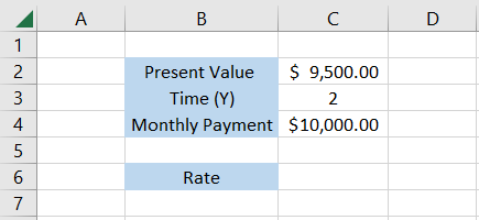
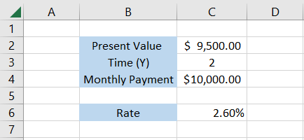
To calculate the interest rate, we will use the formula =RATE(C3,0,-C2,C4,0), which gives the result of 2.60%.
Of course, the dynamics here change entirely compared to the INTRATE function since there is no settlement date or maturity date. However, if we were still to use the INTRATE to calculate the interest rates, we could make some assumptions for the function to work.
Since the holding period is two years, we will assume that today is the settlement date, i.e., 17th January 2023, while the maturity date is 17th January 2025.
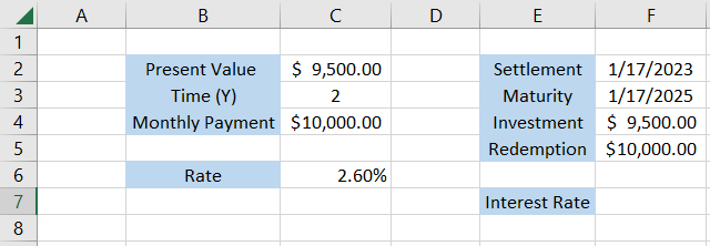
The investment and redemption values remain the same, i.e., $9,500 and $10,000, respectively. Thus, the interest rate will be calculated using the formula =INTRATE(F2,F3,F4,F5), which gives the result:
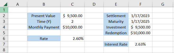
Thus, with a minor tweak in the data representation, even INTRATE can be used to calculate the interest rate of an investment similar to the RATE function.

Free Resources
To continue learning and advancing your career, check out these additional helpful WSO resources:


or Want to Sign up with your social account?