IPMT Function

What is the IPMT Function?

The IPMT function is one of Excel's financial functions. This function returns the money paid in the form of interest from the total payment transacted at the beginning or end of each period.

The precise origins of the IPMT function are tied to the evolution of financial functions within spreadsheet software.

The concept of separating interest and principal portions of loan or investment payments has long been used in financial analysis and planning. Spreadsheet software aims to provide users with a convenient tool to perform such calculations automatically.

Microsoft Excel, one of the most widely used spreadsheet programs, introduced the IPMT function as part of its financial functions suite. With each new version and release of spreadsheet software, including Excel and other programs, enhancements were made to the financial functions, including IPMT.

These improvements focused on increasing the accuracy, flexibility, and ease of use of the function, allowing users to perform complex financial calculations more efficiently.

Over the years, the IPMT function has become a common tool for financial analysis, loan amortization, investment analysis, and other related calculations. It has been widely adopted by professionals in various fields, including finance, accounting, banking, and investment management.

Financial functions in Excel are functions that perform various financial calculations to gain insight into the financial health of a company.

Essential information related to a company's finances, such as cost-to-profit ratios, balance sheets, and debt-paying ability, can be calculated using the financial functions in Excel.

These functions help manage the financial activities and resources of a company.

Finance is the most essential part of a company. Without adequate financial resources, no company can run smoothly in the long run.

Hence the financial functions in Excel are essential for businesses. One such financial function in Excel is the IPMT function, which we will discuss today in this article.

Understanding IPMT Function in Excel

If an individual or company wants to borrow money, they have numerous options to explore, which will depend on various factors.

The interest rate, whether it is compounded monthly or annually, and the total amount of interest needed over the original loan amount are some of the deciding considerations.

Any individual or company that wishes to get a loan would want to get the loan at the lowest interest rate possible so that they have to return a lesser amount of money as interest payment.

This interest payment calculation is done using the IPMT function in Excel.

As discussed earlier, it is one of the financial functions in Excel. The IPMT function in Excel returns the money paid in the form of interest from the total payment transacted at the beginning or end of each period.

When we take out a loan, we must pay back the principal amount and the interest from the time we borrowed the money. Due to the interest we pay, the amount we must return is more than the amount we borrowed in principal.

It computes the portion of the total payment paid as interest for a given loan amount and the period for which the money is borrowed.

We can calculate the interest amount paid for the first, last, or any period in between using the IPMT function in Excel.

Financial analysts are often interested in knowing the principal and the interest component of loan payments for any particular period to draw various insights about the debt schedule.

IPMT Function Formula

They use the IPMT function in Excel to do so. The syntax for using this function in Excel is as follows:

=IPMT(rate, per, nper, pv, [fv], [type])

This formula calculates the interest amount based on the amount of loan due and the period. The terms in parentheses are called the arguments of the function. These are the values required to do the desired computations.

The arguments required by the IPMT function in Excel to produce the desired results are:

• rate is the interest rate for each period.
• per is the number of periods for which the principal amount is demanded. 
• nper is the total number of periods. 
• pv is the present value of the loan or investment. 
• fv refers to the future value of the loan or investment. 
• type is an integer argument whose value is 
  • 1 if the payments are made at the start of each period
  • 0 if the payments are made at the end of each period

The default value of both these arguments is 0. If we do not specify these, it takes the default value, 0. All the remaining arguments are required to perform the calculations.

IPMT Function Examples

Having looked at the theoretical definition and meaning of the IPMT function, let us now see some examples to demonstrate its usage and application of it.

Example 1

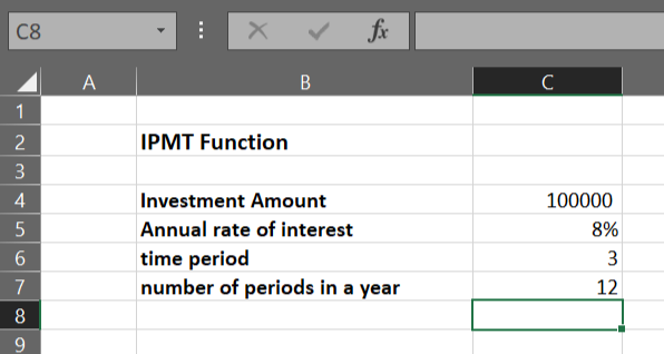
Suppose Mr. Smith took a loan of $100,000 from a bank at an annual interest rate of 8% for three years. There are 12 periods in a year. The data looks as illustrated below:

We wish to calculate the interest payments for the first period using the IPMT function in Excel. To do so, we use the following formula:

=IPMT(C5/C7, 1, C6*C7, C4)

Here, Mr. Smith makes monthly payments, so we need to convert the annual interest rate to the monthly rate of interest, which is (8/12)% (or cell C5/C7), as there are 12 months in a year. This is the value of the argument rate.

We need to calculate the number of periods monthly. The total period of borrowing is three years. There are 12 periods in a year. So the monthly number of periods is 3*12, which is cell C6*C7. This is the nper value.

Here 1 refers to the period for which we calculate the interest amount. Since we wish to calculate the interest amount paid in the first period, we take the value of argument per as 1. For calculating the interest amount in the second period, the value of per will be 2, and so on.

As we have not mentioned the value of arguments fv and type, Excel assumes the default value for these, which is 0. Cell C4 represents the present value of the loan or the argument pv.

On using the above formula in cell C9 of our Excel worksheet, we get the following result:

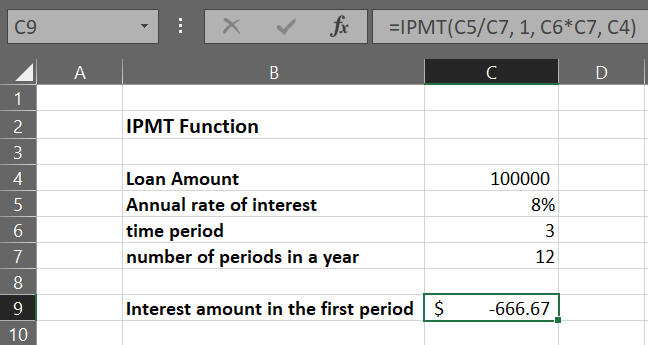
Here, the interest amount returned is negative because there is a net cash outflow, which means Mr. Smith has to give away money to repay the loan. A negative sign would come whenever there is a cash outflow, which signifies a loss of money.

If there is a cash inflow, which means Mr. Smith would have received the interest payment periodically as returns on some investment, the result would have been positive, as shown in the next example.

Example 2

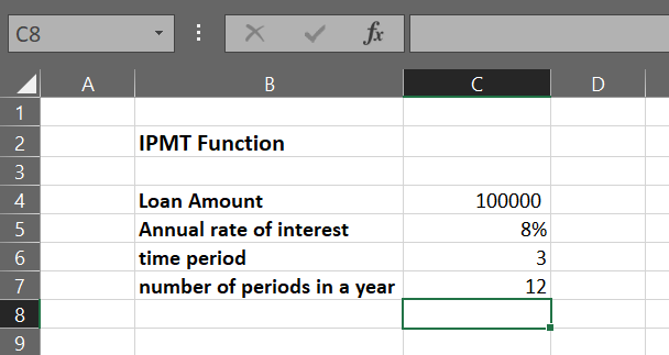
Let us consider the same example 1 as discussed above, but now Mr. Smith, instead of borrowing money, invested $100,000 at an annual interest rate of 8% for three years.

To calculate the interest earned by Mr. Smith in the first period, we would use the following formula:

=IPMT(C5/C7, 1, C6*C7, -C4)

Using the above formula in cell C9 of our Excel worksheet, we get the interest amount received in the first period.

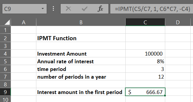
The interest amount above is positive as there is a net cash inflow, which means Mr. Smith earns the interest amount periodically.

In this way, we can calculate the interest amount for any period using the IPMT function in Excel.

Researched and Authored by Devang Shekhar | LinkedIn

Reviewed and Edited by Mohammad Sharjeel Khan | LinkedIn

Free Resources

To continue learning and advancing your career, check out these additional helpful WSO resources:

• HYPERLINK Function
• IFERROR Function
• ISERROR Function
• LOWER Function
• MATCH Function