LOWER Function
One of the Text Functions in Excel that converts all the letters in a text string to lowercase letters.


What is the LOWER Function?
The LOWER function is one of the Text Functions in Excel that converts all the letters in a text string to lowercase letters.
When you type something in Excel, you have complete control over what to input in the selected cell. This includes whether the beginning letter should be capitalized, the entire text string should be capitalized, or the text string should be lowercase.
You would ask - “If we already have control over what case to type in text strings, why does Excel have a function that returns text strings in lowercase?”
The answer is quite simple. Sometimes a third-party website might provide you with files where the text strings need to be in the acceptable format, such as all letters capitalized.
If I were to see such a file personally, I wouldn’t be able to focus on what the data is saying. It would be like the file is screaming at me.
This is where a function such as LOWER can come into play, turning the supplied text strings into lowercase versions.
This article will guide you through the function's syntax, how to use it, and a few examples.
Key Takeaways
-
The LOWER function is a Text Function in Excel that is used to convert text to lowercase letters.
-
Users provide a text string as the argument to the LOWER function, which returns the string with all letters converted to lowercase.
-
Potential errors that users might encounter when using the LOWER function, such as providing non-text values or referencing cells with incorrect data, and how to address them effectively.
-
The LOWER function finds applications in data analysis tasks, such as text mining, text matching, and data visualization, by ensuring that text data is formatted consistently for accurate analysis and interpretation.
Understanding The LOWER function
The LOWER is categorized as a Text function that converts the supplied text string into its lowercase version.
For example, suppose you have the text strings as ‘DOGeCoin.’ If you use the function on this text string, the result would be ‘dogecoin.’
Even though we have capitalized letters in the text string, the result has all the letters in lowercase.
What if we had two text strings separated by a space character? Would the function still work?
Actually, yes.
Suppose you have another text string as ‘Elon Musk.’ Then, using the LOWER function, we would get the result as ‘elon musk.’
It is generally expected to keep at least the first letter of a text string as capitalized. However, the function overrides this expectation and returns the entire text string in a lowercase version.
LOWER Function Formula
The syntax for the function is
=LOWER(text)
where
Text (required) is the reference to the text string, which will be returned in the lowercase version.
As stated earlier, the function completely ignores numerical values, punctuation, and space characters when referencing a text string. So if you have the text string as ‘2341 Avenue, NYC, 14051,’ then the resultant text string would be ‘2341 avenue, nyc, 14051.’
The only things that changed were capitalized letters, while the rest remained the same.

How to use the LOWER Function in Excel?
The function is easy to use because it has only one argument, which can either be hardcoded or a single-cell reference.
The function does accept multiple cells or a range of cells in the argument but will eventually return the first value in the lowercase version.
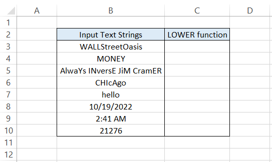
Suppose that you have data in Excel, as illustrated below:
To use the function as a worksheet formula, we will begin with an equal sign, followed by the function name, and finally, input the arguments in column B inside the parentheses.
The formula will be =LOWER(B3) in cell C3 and drag it down to cell C10, which gives the result:
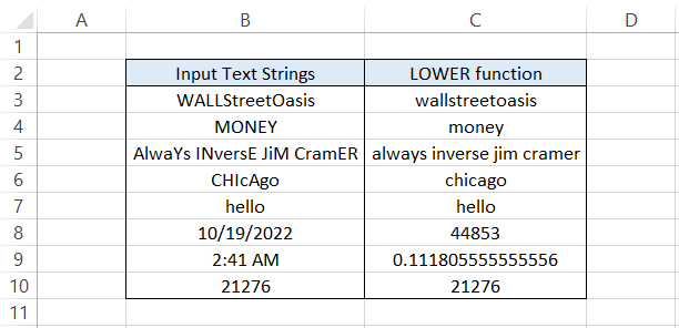
As you can see, whenever we have a text string either in lower case or upper case or even a combination of both, the function will always return the result in lowercase.
The result reveals an interesting change in format for date and time values. Previously, the date was represented in MM-DD-YYYY format, but after using the function, we get the serial number corresponding to the date.
Similarly, we get the fractional equivalent for the time represented in the decimal number. You can also see these formats when you press the Ctrl + ~ key on the keyboard. The bottom line is that these values lose their formatting when you use the function on them.
Finally, the function does not have any effect on numerical values since the function primarily works only on text strings.
LOWER Function Examples
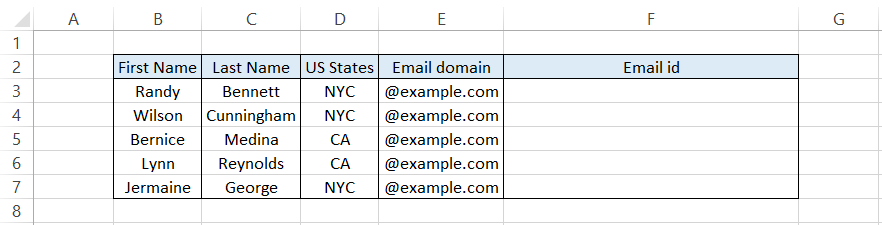
In your daily life, you might use the LOWER function. For example, if you are the HR Manager, you should generate organization email ids for those who recently joined the team.
Concatenation and LOWER function
Suppose three people join an Investment firm’s New York office while two join the California office. The data looks as illustrated below:
If you wanted to create their email ids based on the data available, we would use the formula =LOWER(B3)&LOWER(C3)&"-"&LOWER(D3)&E3 in cell F3 and drag it down till cell F7, which gives the result:
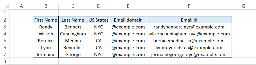
Wherever we have a text string containing capitalized letters, we get lowercase results. Many concatenations also go behind the scenes, such as combining the text strings in columns B, C, D, and E.
We also add the character '-' that separates the full name from the state where the office is located.
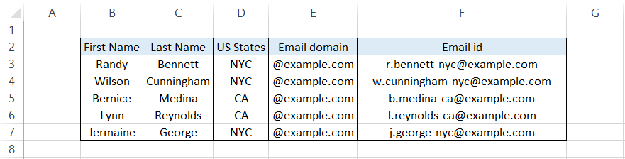
Although it's not wise to create organizational email IDs based on only single first or last names(for example, [email protected] or [email protected]), you can still use the LEFT text function to extract those particular text characters from the result.
For example, we can use the formula =LEFT(LOWER(B3),1)&"."&LOWER(C3)&"-"&LOWER(D3)&E3, which will give us the email ids in [email protected] format.
If you become good with concatenation and text functions, text manipulations and data analysis would be a park walk!
Flash Fills
Though this is not a direct application of the LOWER function, it acts as an alternative instead of using the coveted function that returns the text string in the lowercase version.
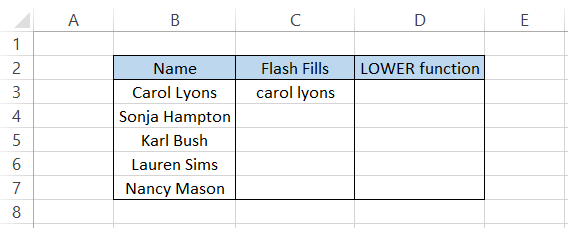
Suppose you have the data in Excel, as illustrated below:

We will type in the full name in a lowercase version to use the flash fills. So, for example, Carol Lyons becomes ‘carol lyons’ in cell C3.
After this, all you need to do is press the Ctrl + E in cell C3, which gives the result:
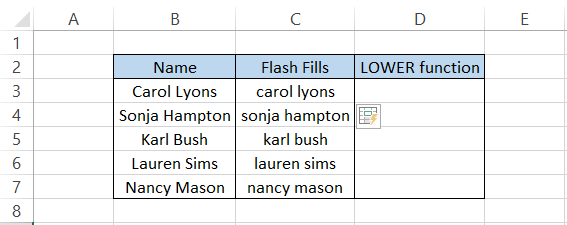
If we were to use the =LOWER(B3) formula in cell D3 and drag it down till cell C7, we would get the same result as
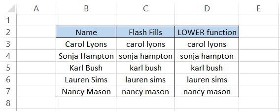
You can use the method that best suits your requirement, i.e., either flash fill or the function. However, the function would always have the upper hand when building Excel models with intricate formulas.
LOWER vs. UPPER function
If we have a function that changes a text string to its lowercase version, then it's obvious we would have another function that works exactly.
The UPPER is categorized as a text function that will return the given text string in capitalized version or the upper case.
For example, if you have a text string as ‘Apple Inc,’ the function will return the result as ‘APPLE INC.’
All the existing capitalized letters are unaffected, while the letters which are in lowercase will immediately return to the capitalized form.
The function does not affect numerical values or any other special characters.
The syntax for the function is:
=UPPER(text)
where,
text - (required) the reference to the text string, which will be returned in the capitalized version.
Example
Let’s see an example of how the results differ for UPPER and LOWER functions.
Suppose you have the data in Excel, as illustrated below:
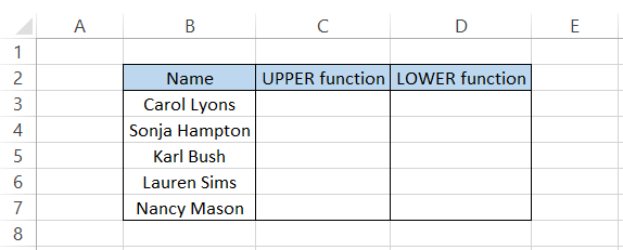
To get the result in uppercase, we will use the formula =UPPER(B3) in cell C3 and drag it down to cell C7, which gives the result:
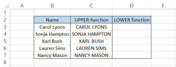
Irrespective of whether the letters are capitalized or in the lowercase version in the referenced text string, we ultimately get the result in uppercase.
Similarly, we will use the formula =LOWER(B3) in cell D3 and drag it to cell D7, which gives:
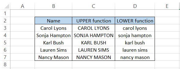
Either function can be used when you return the text strings in lower or upper case.
LOWER vs. PROPER function
The PROPER function is perhaps one of the greatest creations in Excel’s history since its launch in 1985.
We all had those instances when the files downloaded from third-party websites did not have the data in ‘proper’ formats.
The PROPER is categorized as a text function that takes a text argument and returns the first letter of a word in uppercase while the rest of the letters are set to lowercase.
For example, if you have the text string as ‘ELON MusK, the PROPER function returns the result as ‘Elon Musk.’
The syntax for the function is:
=PROPER(text)
where
text = (required) a text string enclosed inside the quotation marks, a cell reference for the text strings, or a formula that returns a text value.
Example
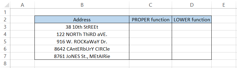
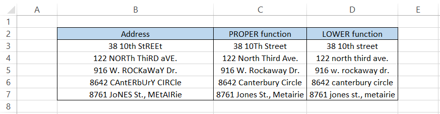
An in-depth comparison example would help us better understand how the results for the PROPER and LOWER function differ. For example, suppose you have some addresses in Excel, as illustrated below:
To get the street address in the ‘proper’ format, we will use the formula =PROPER(B3) in cell C3 and drag it down to cell C7, which gives the result:
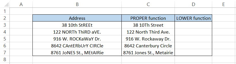
As you might have already noticed, all the unnecessary capitalized letters get replaced by a lowercase version except for the first letter in the text string.
If there are numerical values, special characters, or spaces between the text strings, the counter gets reset, and the substring, again, begins with a capital letter.
On the other hand, by using the formula =LOWER(B3) in cell D3 and dragging it to cell D7, we get the text strings in the lowercase version, as illustrated below:
VBA code that returns text string in lowercase
You can write a VBA code that will return the text strings in lowercase—for example, copying the text in column A to return the lowercase text string in column B.
Another way could be by selecting a range of data and then running the code, which ultimately gives us the expected result.
In this section, we will explore the latter example of VBA code, i.e., running the code by selecting a range of values in Excel.
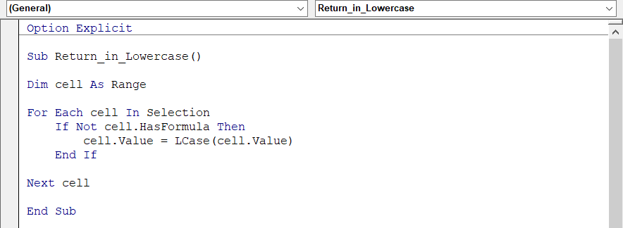
The snippet of code that we will use is illustrated below:
To run the code, you must select the range of cells, go to the Developer tab and then run the macro.
However, you can also create a button from the Developer tab and assign a macro to it to use the VBA code directly.
However, a VBA button does take up unnecessary space in the spreadsheet, right? So instead, you can create a button on the ribbon, which you can directly press to run the macro.
The steps you need to follow are:
-
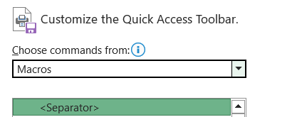
Click on File > Options > Quick Access Toolbar
-
Select ‘Macro’ under the Choose commands from the drop-down menu.
- You will see all the different VBA codes that you have written. Next, select the one you intend to add to the ribbon, which in this case is Return_in_Lowercase(this is the same name we used while writing the code).
- Click on Add to move the macro. You can also edit the icon for the macro based on what the code does by clicking on ‘Modify.’ For example, we changed the icon to
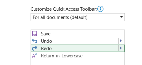
- Finally, click on Ok, and you will find the icon for the macro in the ribbon.
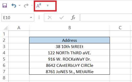
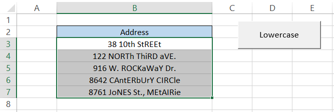
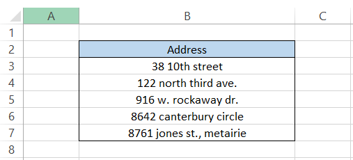
Now, select the range B3:B7 and click on the icon to run the macro. You will get the result as
This trick is quite handy when you run a particular snippet of VBA code daily or rather frequently.

Free Resources
To continue learning and advancing your career, check out these additional helpful WSO resources:


or Want to Sign up with your social account?