MROUND Function

What is the MROUND Function?

The MROUND, in simple terms, can be explained as a function that returns the rounded value, which is the multiple of the number we input in Excel.

We have already seen enough rounding functions in Excel, such as ROUND, ROUNDUP, and ROUNDDOWN. Let me guess, you have already decided that you will never use it in real-life scenarios.

You are wondering why Excel needed to come up with another function that sounds complicated yet is extremely easy to use.

Why you need such a function depends entirely on the use case and the scenario you are working on. However, having an additional cannon in the arsenal will never hurt.

In this article, we will see the MROUND function, how to use it, and a couple of examples to understand it better.

Understanding The MROUND Function

The MROUND is categorized as a Math and Trigonometric function that converts the user-input number into the nearest multiple of the number which needs to be rounded.

For example, suppose that the number you want to round equals 9. Let’s say you need 9 to be rounded off by a number that is a multiple of 2.

If you check all the multiples of 2, i.e., 2, 4, 6, 8, 10… then there are two multiples near 9, which are 8 and 10. Both are equidistant to 9, yet Excel will return the result as 10 as the number gets rounded up.

However, if the base number for multiple is changed to 4 to give multiples 4, 8, and 12, the result is returned as 8 since it is closer to 9 than 12. In such a case, the number gets rounded down.

The syntax for the function is

=MROUND(number, multiple)

where

• number - (required) the number which will be rounded off.
• multiple - (required) another number whose multiple will be returned as the rounded value.

Next, let's see a simple example of using the Excel function.

How to use the MROUND Function in Excel?

A simple syntax makes using the MROUND function even easier. It wasn’t like other rounding functions were complicated to use; the same followed with MROUND and hopefully follows for all the related functions in the future.

All you need to do is begin with an equal sign, type in the function name and finally input the arguments inside the parentheses.

a. Example #1

For example, suppose you have the data as illustrated below:

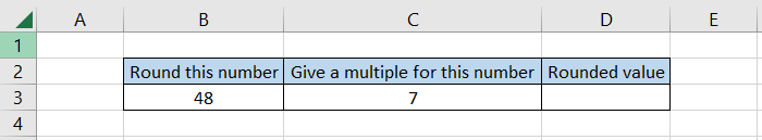
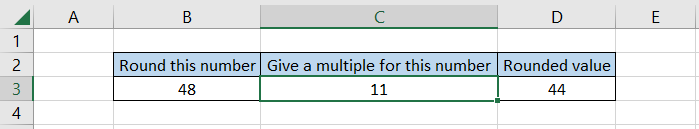
Here, we will use the formula =MROUND(B3,C3) in cell D3, which gives the result of 49. Based on all the multiples of 7, the nearest one to the number 48 is 49. Hence the number gets rounded up in the process.

If the number in cell C3 was changed to 11, the rounded value in cell D3 would be 44 since 44 is far closer to 48 than 55. Based on what multiple of the number is closer to the target number, we either get a rounded-up or round-down value. 

b. Example #2

Let's take a number and find different rounded numbers using different values as a base number for multiple.

Suppose you have the data as illustrated below:

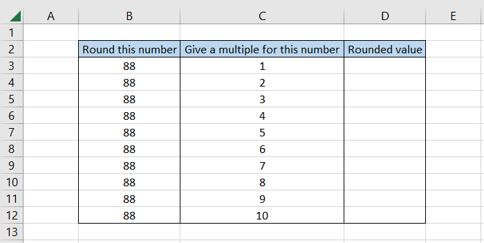
We will use the formula =MROUND(B3,C3) in cell D3 and drag it down to cell D12, which gives the result:

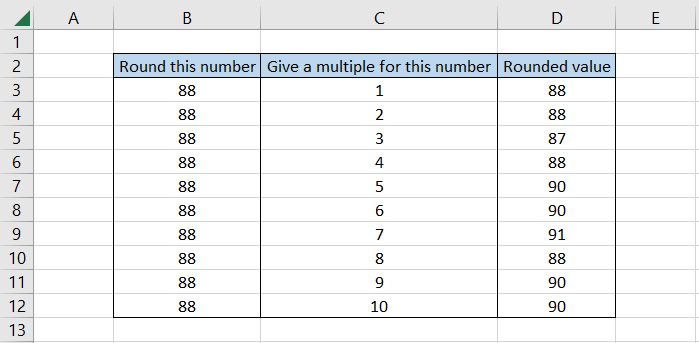
Interpretation:

1. The multiple of 1 and 2 that comes closest to the number 88 is 88 itself.
2. For number 3, the nearest two multiples are 87 and 90. The former is one number away, while the latter is two numbers away from 88. Thus, the number gets rounded to the nearest, i.e., 87.
3. The same case follows for all the numbers up to 10, wherein the rounded value is 90 since it is far closer to 88 than 80.

c. Example #3

Would the function work for decimal numbers or other data stored as numbers? We believe you might have had the same question while reading the article.

The function works on all the datatypes stored as numbers in Excel. This includes natural numbers, decimal numbers, and even date and time values.

We are already aware that date and time values are stored as serial numbers and decimal numbers, respectively, so it ticks off the necessary criteria of being a numerical value.

Suppose you have the data as illustrated below:

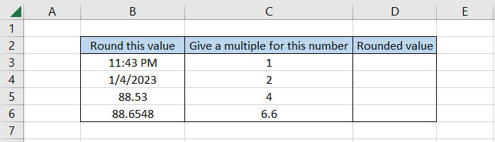
Here, we will use the formula =MROUND(B3,C3) in cell D3 and drag it down till cell D6, which gives the result:

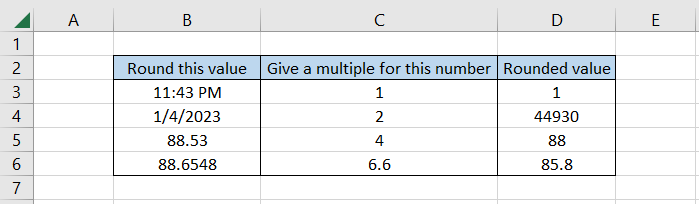
Interpretation:

1. For the time value 11:43 PM, if we check the decimal counterpart, we find that the value equals 0.98819. So the closest multiple to it is ultimately 1, the exact same result returned using the function.
2. The serial number for the date 4th January 2023 is 44930. Since it is divisible and multiple of 2, we get the same number in cell D4.
3. When a decimal number such as 88.53 needs to be rounded towards a multiple of another number 4, Excel's alternatives are 84, 88, and 92. Amongst those, the one that comes nearest to the given number is 88.
4. In cases where both the numbers are decimals, the rounded value is also returned as a decimal number, which is 85.8.

MROUND vs. ROUND function

The ROUND function is categorized as a Math and Trigonometric function that rounds a given number to ‘n’ decimal places.

Based on the digit in the ‘nth’ decimal place, the number either gets rounded up or rounded down in Excel.

For example, if you have the number 18.1236 and round it to two decimal places, the result would be equal to 18.12, whereas if the number is rounded to three decimal places, the result is 18.123.

The rounding works on a simple principle as opposed to MROUND, i.e., when the digit to the right of the ‘nth’ place is between zero and four, the number gets rounded down.

On the other hand, if the number lies between five and nine, the number gets rounded up, as we saw earlier.

The syntax for the ROUND function is

=ROUND(number, num_digits)

where,

• number - (required) the number which will either be rounded up or down
• num_digits - (required) the ‘nth’ place up to which the number will be rounded

Suppose you have the data as illustrated below:

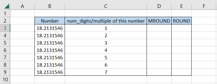
To get the rounded value based on multiple, we will use the formula =MROUND(B3,C3) in cell D3 and drag it down to cell C9, which gives the result:

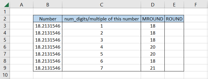
Similarly, we will use the formula =ROUND(B3,C3) in cell E3 and drag it down till cell E9, which gives a rather contrasting result as

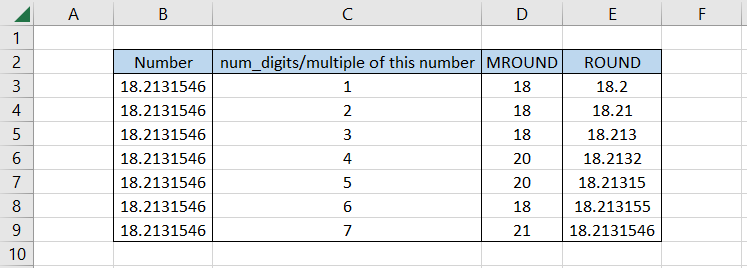
If we speak of accuracy, ROUND is the best option to return rounded numbers up to whatever ‘nth’ place you require. If you need rounded values in multiples, then MROUND is the alternative you can opt for.

ROUNDUP Vs. ROUNDDOWN function

You need to remember that the two other rounding functions are ROUNDUP and ROUNDDOWN.

The ROUNDUP function generally rounds a number away from zero, whereas the ROUNDDOWN reduces the ‘nth’ decimal digit in a number by rounding toward zero.

Earlier, we saw that the ROUND function works on criteria where it rounds up a number between five and nine, whereas it rounds down when the number lies between zero and four.

However, the same criteria do not apply to these two functions.

Irrespective of whether the number lies between those two intervals, the ROUNDUP function will always round a number away from zero, while the ROUNDDOWN will round a number towards zero.

Both functions have similar syntaxes as

=ROUNDUP(number, num_digits)

Or

=ROUNDDOWN(number, num_digits)

where,

• number - (required) the number which will be either rounded up or down
• Num_digits - (required) the ‘nth’ digit upto which the given number will be rounded up or down

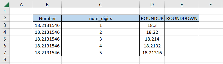
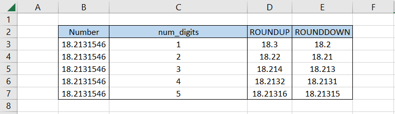
Suppose you have the data as illustrated below:

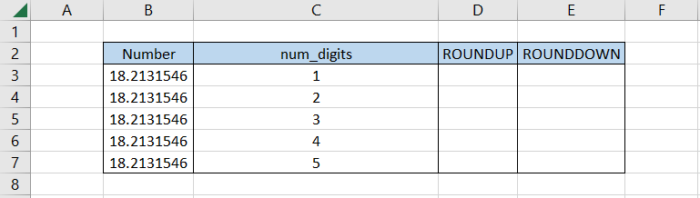
When we use the formula =ROUNDUP(B3,C3) in cell D3 and drag it down till cell D7, we get the result:

Similarly by using the ROUNDDOWN function formula =ROUNDDOWN(B3,C3), we get the result:

Finally, now you can decide whether you want a rounded value using the function that:

1. Uses multiple of another number
2. Based on general rounding criteria
3. Always rounds up or rounds down a given value

Free Resources

To continue learning and advancing your career, check out these additional helpful WSO resources:

• MATCH Function
• OFFSET Function
• ROW Function
• INDIRECT Function
• TRANSPOSE Function