NORMDIST Function
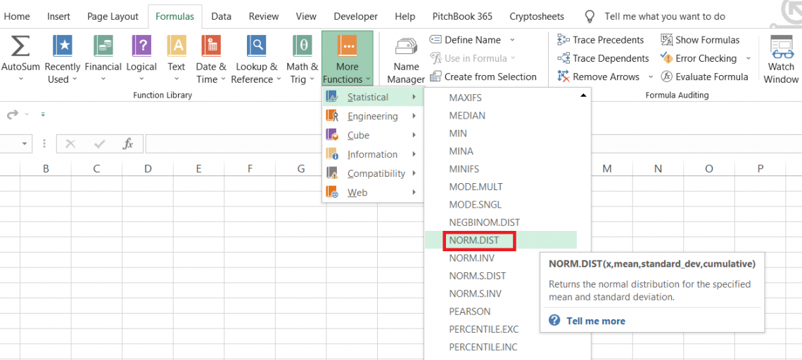
An Excel Statistical function that calculates the probability density function (PDF) and cumulative distribution function (CDF) for a normal distribution using the given mean and standard deviation.


What is the NORMDIST Function Excel Normal Distribution?
The NORM.DIST function is an Excel Statistical function that calculates the probability density function (PDF) and cumulative distribution function (CDF) for a normal distribution using the given mean and standard deviation.
The NORM.DIST function helps in the analysis by providing insights into the normal distribution of data, which can be useful in risk assessment, decision-making, and probability calculation.
We know you have many questions about all those complicated concepts and statistical jargon. But first, we need to understand what a normal distribution is.
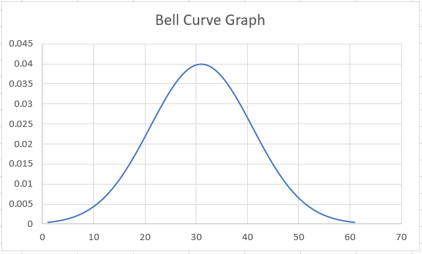
A normal distribution is a bell-shaped graph where most values are concentrated around a central region and recede in numbers as we leave the center.
Some standard distribution variables are height, birth weight, SAT scores, blood pressure, or even measurement errors.
A normal distribution can take any value for its mean and the standard deviation. In this graph, as you might have observed, the data near the middle(mean) is far more than the ends, where the chart tapers towards zero.
- The NORM.DIST function calculates the probability density function(PDF) and cumulative distribution function (CDF) for a normal distribution using the given mean and standard deviation.
- The NORMDIST function returns a probability value between 0 and 1. If cumulative is TRUE, it returns the cumulative distribution function (CDF) at x. If cumulative is FALSE, it returns the probability density function (PDF) at x.
- The NORMDIST function is commonly used in statistics, probability theory, and financial modeling to calculate the probability of a specific value occurring within a normal distribution.
- The NORMDIST function may return errors if any of the arguments are non-numeric or if standard_dev is zero. In such cases, it may return a #VALUE! error.
Understanding NORM.DIST function
The NORM.DIST is categorized as a statistical function that calculates the values for the probability density function and the cumulative distribution function based on the boolean value you input.
For example, when you have the given number(x) as equal to 29, you use NORM.DIST function, you get the result as 0.000968 and 0.000327, respectively, as cumulative density function and probability density function.
The syntax for the function is:
=NORM.DIST(x, mean, standard_dev, cumulative)
where,
- x - (required) the input value for which we are calculating the distribution
- mean - (required) the center value of the distribution
- standard_dev - (required) the standard deviation of the dataset
- cumulative - (required) boolean value determines whether the function will calculate the probability density function or the cumulative density function.
If the value is equal to TRUE, the function calculates the cumulative density function, whereas if it is FALSE, the result would be the probability density function.
Let's see how to get both values in Excel and how those values can be helpful in professional life.
Note
The NORMDIST function was replaced by NORM.DIST in Excel 2010 has been present in all the versions ever since. The former function is still current in Excel as a compatibility function. However, both parts perform the same task and return the same result.
Probability Density Function
The Probability Density Function defines the relationship between a variable and its probability in such a way that the function enables us to find the possibility of the variable.
A variable can be of two different types - discrete or continuous.
Discrete Variables
When the variable can take only a finite number of values within a specified range, it is called a discrete variable. For example, head or tales on two different coins. Tossing both coins can result in either a head, tail, or a head-tail combination.

The combinations would not exceed four, whereas the sides of the coin can be only two, i.e., the values are finite.
2. Continuous variables
On the other hand, a variable that can take an infinite number of values within a specified range is called a continuous variable. For example, assume the person's height. We know that it is 157cm, but in reality, it could also be 157.0011cm or 157.13548cm.
The best you can do is only define the range where the value falls in and can take an infinite number of values.
Suppose you plot a probability density function for a continuous random variable n.' Let's say you want to find the area between the probability points x and y, as in the graph illustrated below:
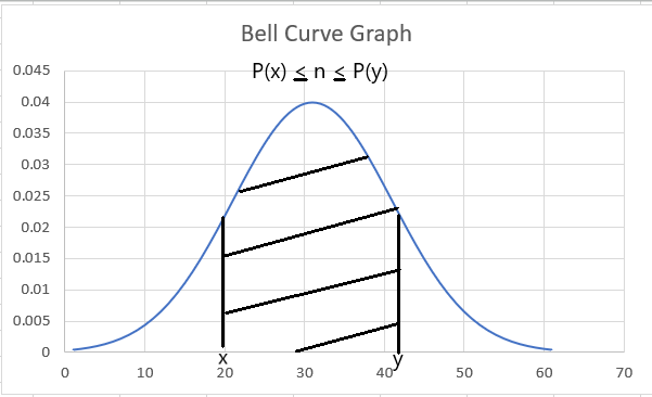
The area between the two points, i.e., the size of the curve, can be represented as
P(x) <= n <= P(y)
Suppose you have the graph for the probability for 'n' as illustrated below. The x-axis represents the range of values, while the Y-axis has the probability density function.
Finding the area to the left of the graph can give the probability that the value is 20.
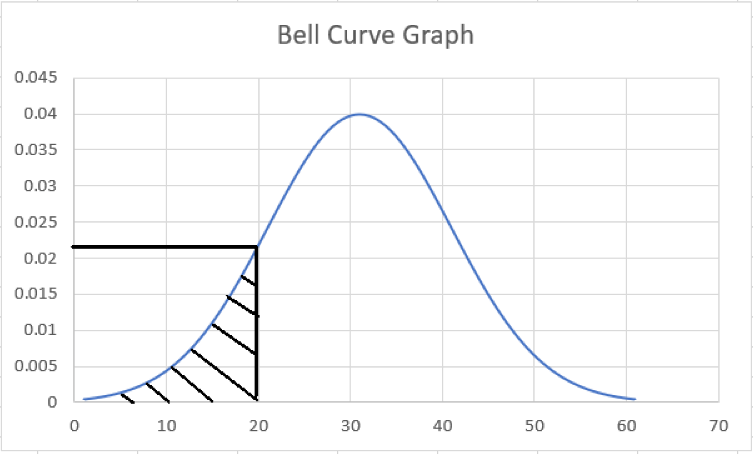
For example, as in the graph illustrated above, the probability of a value being 20 is less than or equal to 0.022. It is represented by equation P(n= 20) <= 0.022.

Cumulative Density Function
The Cumulative Density Function describes the probability distribution of the random variable 'x'. Similar to the probability density function, it can calculate the probability of discrete and continuous variables.
The graph plotted for the Cumulative Density Function is obtained by summing up the probability density function to get the cumulative probability for the random variable.
What do you mean by cumulative? An example would probably help to explain this better. For example, let's say the first value is 1 and the second is 3; the cumulative value will be 4. If the next value is 2, then the cumulative value is 6.
The next value in the series gets added to all the previous values to give the final deal. Based on this, you can probably imagine what kind of graph you would get for the Cumulative Density Function.
The graph will begin at zero probability and level down around the probability value of one.
These statistical concepts are vast but immensely useful. Let's stick to the basics for now as to how the graphs for either density function look and proceed with the NORM.DIST function!

NORMDIST Function Example
There won't be many instances of using functions such as NORM.DIST unless you are specifically working on projects based on statistics.
As we know, the normal distribution can accept all the mean and standard deviation values.
The question is, how do you calculate the density values and plot them on the graph?
Suppose that you have a dataset for height, as illustrated below:
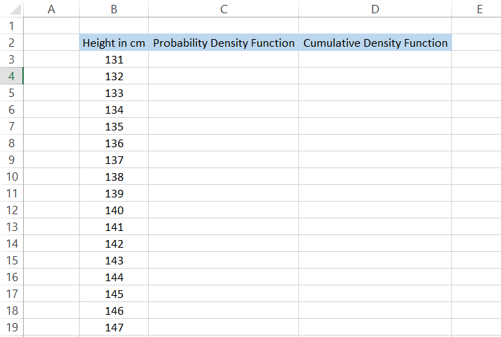
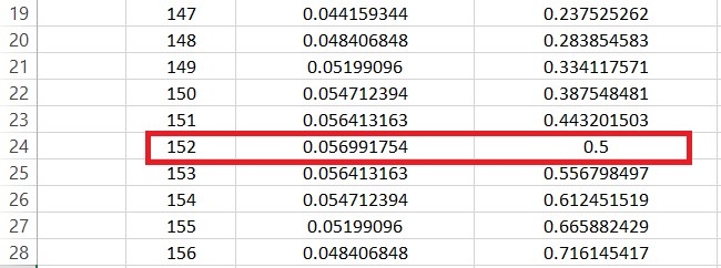
The size starts from 131 cm and ends at 176 cm in the column. The mean size we have assumed is 152 cm, and the standard deviation is 7cm.
You can also use the formula Mean - (3 * Standard Deviation) to get the first height, i.e.,
152 - (3 * 7), which gives us 131 cm.
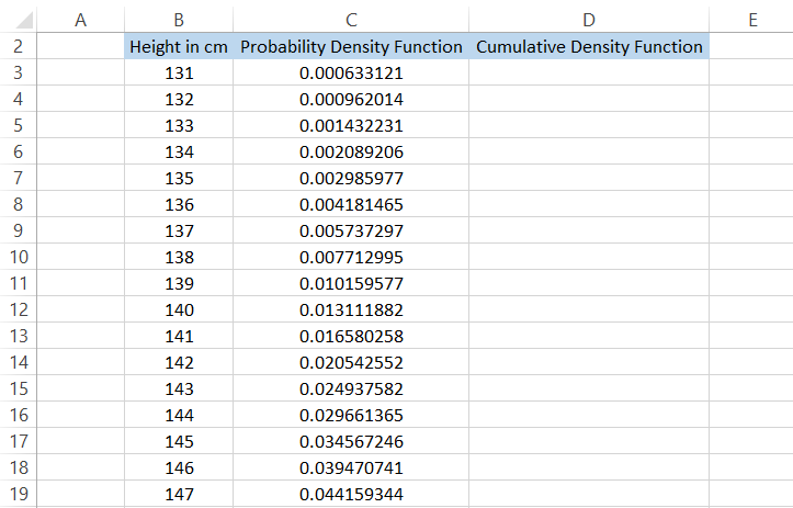
We will use the formula =NORM to calculate the probability density function.DIST(B3,152,7, FALSE) in cell C3 and drag it down to the last cell, which gives the result.
On the other hand, to calculate the cumulative density function, we will use the formula =NORM.DIST(B3,152,7, TRUE) in cell D3 and drag it down to the last cell to get the result:
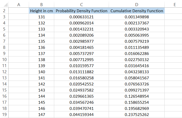
One observation you would make from these values is that the probability density function will have a maximum value at the mean value, i.e., 152. In contrast, the cumulative density function would have a probability of precisely 0.5.
But the question remains - how do you draw the graphs for the respective density values?
First, select the entire data in columns B and C.
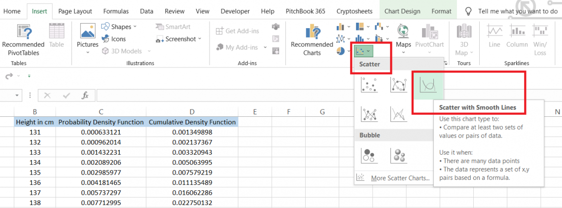
Click on Insert > Charts Section > Scatter charts > select the option for ‘Scatter with Smooth Lines.’
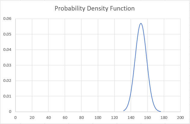
This will display the graph for the probability density function, as illustrated below:
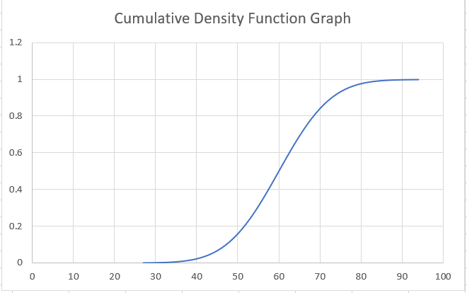
Similarly, to insert the graph for the Cumulative Density function, we will select the entire data in columns B and D and select the Scatter chart with smooth lines.
We get the graph as illustrated below:
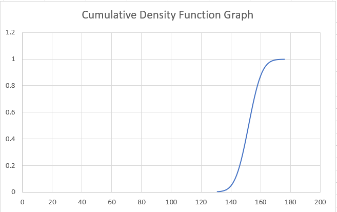
Based on the graph, you can easily find the probability for a variable. For example, the likelihood of a person having a height of around 160cm is approximately 0.8 - 0.9
Practical Examples Of NORMDIST Function
The NORM.DIST function can primarily help calculate probabilities, even in finance, along with statistics.
In this section, we will see a couple of examples of how you can use NORM.DIST functions in real-life scenarios.
Example #1
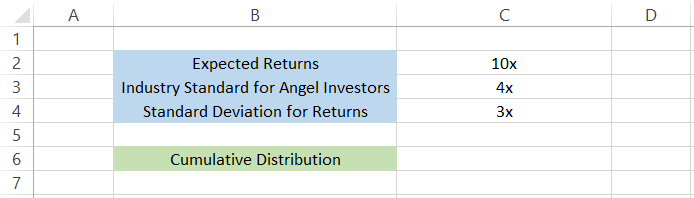
Let's say that you are an angel investor who usually looks for a 10x return on the investment. However, the average industry return for angel investors is around 4x, while the standard deviations in the returns are 3x.
We need to calculate the probability of the returns on the investment at or below 10x. The data so far looks, as illustrated below:
By using the formula =NORM.DIST(C2, C3, C4, TRUE) in cell C6, we get the result as 0.977249868, which roughly equates to 98%. This means that around 98% of the angel investors are making returns below the expected returns of 10x.
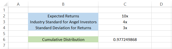
Based on the industry standard (mean value) and the standard deviation, the chances of making 10x returns are around 2%.
Wait, what if you were calculating the probability density function? What would be the interpretation of the result?
The formula you will use to calculate the probability density function is =NORM.DIST(C2, C3, C4, FALSE) gives you the result of 0.017996989.
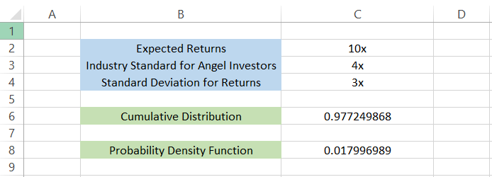
This means that, based on the mean value and standard deviation, only 1.7% of angel investors are making 10x returns on their investments.
Example #2
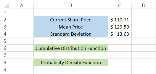
Suppose that you are looking to invest in Alphabet Inc. The current share price of Class A common stock as of 9th September 2022 is $110.71.
The average closing price for the past year is $129.59, calculated based on the historical price change dating back to 9th September 2021.
The standard deviation for the population is $13.63, which again is calculated using the STDEV.P function in Excel for the past year's price. The data so far is, as illustrated below:
We will use the formula =NORM to calculate the Cumulative Distribution function.DIST(C2,C3,C4,TRUE), which gives us the result 0.082999 or 8.3%
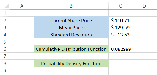
This means that there is an 8.3% probability that the current price will stay below the mean cost of $129.59 or; in other words, the chances of the Alphabet Inc stock price going over the mean price of $129.59 is a whopping 91.7%
Similarly, we can find the probability density function using the formula =NORM.DIST(C2,C3,C4,FALSE), which gives the result 0.011214 or 1.12%.
This means that there is a 1.12% chance of the stock staying at the current price of $110.71
Example #3
Suppose you take up a 30-day net profitable challenge as a day trader. The profit and losses that you make each day are, as illustrated below:
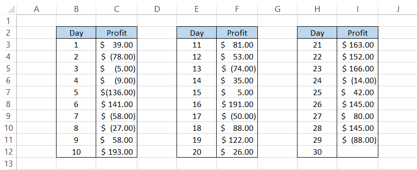
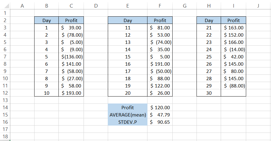
Let's say you want to make at least $120 on the 30th day of the challenge. The mean value based on all the profit/losses is equal to $47.79, while the standard deviation is equal to $90.65
Again, the cumulative distribution function and probability density function will be calculated using the formula =NORM.DIST(F14,F15,F16,TRUE) and =NORM.DIST(F14,F15,F16,FALSE), respectively.
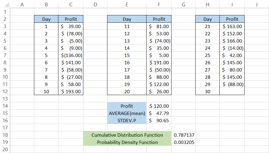
This gives the cumulative distribution function as 78.71%, meaning that the profit will be below $120 based on the probability, while it will be above $120 with a chance of 21.9%
On the other hand, there is a probability of 0.32% that the profit would be equal to $120 based on the value returned for the probability density function.
Free Resources
To continue learning and advancing your career, check out these additional helpful WSO resources:


or Want to Sign up with your social account?