Demand Curve

What Is A Demand Curve?

A Demand Curve shows how the price of a commodity affects its demand in a graphical format. As such, we can say that the demand curve is a graphical representation of the connection between the price of a commodity and demand for that product at a specific point in time.

In the demand curve graph, the quantity demanded is denoted in the X-axis while the Price is denoted in the Y-axis. 

This curve follows what is known as the law of demand, which states that if the price of goods increases, the demand falls and vice versa (except Giffen and Veblen goods). 

This results in a downward-sloping curve demonstrating an inverse connection between the price of products and services and the quantity required. The degree to which quantity demand falls as prices rise is referred to as demand elasticity or price elasticity of demand. 

Under the price elasticity of demand, the demand can be classified into elastic and inelastic demand. The demand curve itself can be categorized into two types individual demand curve and market demand curve.

Drawing A Demand Curve

A demand schedule is a table that shows various quantities of a commodity demanded at various price levels during a given period. And demand curve is the graphical representation of this demand schedule. 

The demand curve is based on the law of demand, which states that if the price of a commodity rises, its demand will fall, and if the price falls, the commodity demand will rise.

So, based on this law, the quantity demanded has a negative relationship with the price. It is of two types: Individual demand curve and market demand curve.

An individual demand curve shows how an individual changes his demand for a commodity at different price levels. The market demand curve shows how much the market (the sum of the demand of all consumers) is willing to buy a commodity at various price levels. 

The X-axis in this graphical depiction of demand denotes price, while the Y-axis denotes the amount desired (in units).

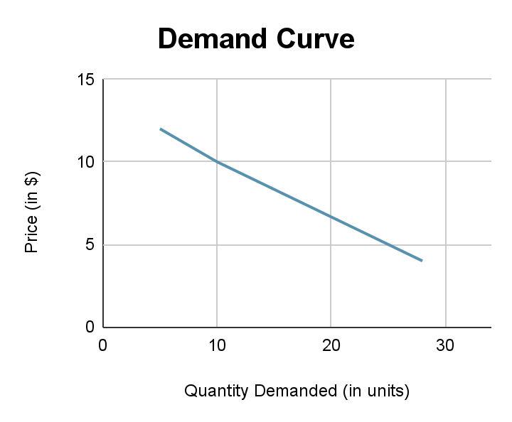
Let us look at an example: 

The table represents the demand schedule in the above example. It shows how much a commodity is demanded at different price points. As seen in the table, the demand falls with the price rise. Now, if we plot this data in a graph, we get a downward-sloping line. 

The formula for the Slope of the Demand Curve is;

Slope of demand Curve = (Change in Price (𝚫P) / Change in Quantity (𝚫Q))

Some important assumptions have to be considered while studying a demand curve. These assumptions are:

• The income of the consumer remains the same
• The price of complementary goods remains unchanged
• The preferences, tastes, habits, and fashions of the consumer remain unchanged
• The number of consumers remains unchanged
• The commodity is a normal good and has no status value
• There is no expectation of a price change in the future

Shifts In The Curve

We know that the Demand Curve shows the relationship between the price and quantity demanded of a commodity, so anytime a variable other than price impacts a commodity's demand in any manner, the curve shifts to left or right depending on the nature of the change.

The curve will shift to the right, showing an increase in demand; if the change in the variable is positive, and If the changes are unfavorable, the curve will shift left showing a decrease in demand.

There are various reasons for this shift; some of these factors are:

1. Change in price of substitute goods
2. Change in the income of the consumer
3. The expectation of change in future prices
4. Change in tastes and preferences 
5. Population change

Let us understand this by looking at a graph.

In the above graph, DD is the original demand curve. So if, say, there is a rise in the income of the consumers, this will allow the consumer to demand more commodities at the same price as they have more income to spare. 

This will shift the curve to the right from DD to D1D1, where at the same price (P), more quantity is demanded (Q1). 

And if there are any negative effects like a drop in population due to war or other natural causes, this will reduce the number of consumers in the market, dropping the demand. 

This will shift the curve to the left from DD to D2D2, where at the same price (P), less quantity is demanded (Q2). 

Movements Along the Demand Curve

When there is a change in the price of a commodity while other factors remain the same, there will be an upward or downward movement of quantity demanded along the curve. It is also known as Expansion in Demand and Contraction in Demand. 

Let us understand this by looking at a graph.

Following the law of demand, the quantity of demand falls when a price increases. And we can see this in effect in the above graph.

When the Price (P) rises to P2, the quantity demanded falls from 0Q to 0Q2, and there is an upward movement in the curve where previously which the price (P) meets quantity demand (Q) “point A” moves to a new point C at price (P2) and quantity demand (Q2).

This upward movement is also known as a contraction in demand, as now there is less demand for the commodity than before. 

When the Price (P) falls to P1, the quantity demanded increases from 0Q to 0Q1, and there is a downward movement in the curve where point A moves to point B, indicating a rise in quantity demand at the price P2.

This downward movement is known as expansion in demand, as now there is more demand do the commodity than before. 

Demand Curves Based On Elasticity Of Demand

The elasticity of demand or price elasticity of demand shows to what degree the demand for a commodity will respond to the change in price.

So, based on the responsiveness of demand to change in price, there are different degrees of elasticities of demand. There are five general categories in price elasticity of demand:

1. Perfectly elastic (Ed = ∞)

A perfectly elastic demand is an infinite demand at a particular price point, and any price change will result in demand going to zero. In the below curve, we can see that the commodity has an infinite demand at the price P.

It is primarily a theoretical concept with very few real-world examples. However, during the 2021 global pandemic, we saw a rise in demand for personal vehicles even though the price was unchanged. 

So we can say that for a brief period, we saw a perfectly elastic demand until the auto industry increased the price.

2. Perfectly Inelastic (Ed = 0)

A perfectly inelastic demand is a situation where the price change does not affect the demand for a commodity. In the below curve, the quantity demand 0Q does not change even if the price changes from P1 to P2.

An example of this type of demand is life-saving medications. Even if the price were to fall, the only people demanding this type of commodity are those who need it and will only buy a certain amount to sustain their lives.

3. Highly elastic (Ed > 1)

Highly elastic demand is a situation where a small price drop can result in a massive increase in the quantity demanded. In the below curve, we can see how a small drop in price from P1 to P2 changed the quantity demanded from 0Q1 to 0Q2.

Examples of this type of demand include commodities like smartphones, computers, or TVs. Most consumers who want to own an iPhone and can’t afford it at the moment will jump at the chance when the price drops as a discount offer.

4. Less Elastic (Ed < 1)

Less elastic demand is a situation where even a large price drop will not affect the demand to the same extent. The below curve shows that a price drop from P1 to P2 increased the quantity demanded to only 0Q1 to 0Q2

We can see this type of demand for products like milk, salt & vegetables. A price drop will increase the demand for milk a little bit, but people will not likely consume more milk than they already consume. 

5. Unitary elastic (Ed = 1) 

Unitary Elastic demand is a situation where the percentage drop in price equals the percentage group in quantity demanded. In the graph below, we can see that the change between P1 to P2 is equal to the change between Q1 to Q2.

This type of demand is mostly seen in commodities like scooters, bikes, refrigerators, etc. 

Exceptions To The Demand Curve

As the demand curve is based on the law of demand, so situations where the law of demand does not work, the curve also loses its property of showing a negative relationship between the price of a commodity and its quantity demanded. 

Some of these exceptions are explained below

Giffen Goods

Inferior goods like bread and rice, which have no direct viable substitute, see their demand rise with the price rise. 

This is because of Giffen’s Paradox, given by Sir Robert Giffen when he observed that low-paid British wage earners would increase their bread consumption with the price rise.

He concluded that as bread is a staple food of working and can not be substituted by any other food, they were forced to cut other food items like meat to buy bread, and to cover the deficit of meat, they would buy more bread at higher prices.

Veblen Goods

Veblen goods are those goods that act like status symbols. As such, this type of goods has a positive relationship between price and quantity demanded. This means the demand will increase with the price rise.

This is because these goods are mostly a sign of wealth and are used as a status symbol, so if the price were to fall, it would lose its exclusivity, and the demand would fall. 

Fear Of Shortage

The law of demand will stop working when there is a fear of a future shortage of a commodity. In the 2021-22 global shutdown, we saw many examples, like toilet paper, face masks, and hand sanitizers breaking the law of demand. 

At the time, even after a massive price increase, the demand was not falling as there was a fear of future shortages, and consumers wanted to stock up before supply ran out.

Researched and authored by Kunal Raj | LinkedIn

Reviewed and Edited by Shahrukh Azim Butt | LinkedIn

Free Resources

To continue learning and advancing your career, check out these additional helpful WSO resources:

• Aggregate Supply and Demand
• Cross Elasticity Demand (XED)
• Demand Theory
• Income Elasticity of Demand
• Quantity Demanded