Aggregate Supply and Demand
The total supply and demand at a specific period and at a particular price in an economy.


What Is Aggregate Supply and Demand?
The aggregate supply and demand is defined as the total supply and demand at a specific period and at a particular price in an economy.
First and foremost, we must understand how the average price of all products and services produced in a country influences total production and total consumer expenditure in that economy.
Following that, the Aggregate Supply is the total supply of products and services enterprises in a country's economy intend to sell during a specific period. It refers to the total number of goods and services a company is ready to offer at a specified price.
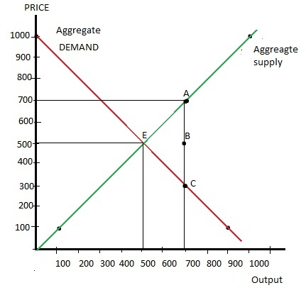
The aggregate supply and demand curve/schedule represents a macroeconomic model that employs aggregate supply (AS) and aggregate demand (AD).
The AD is thus the total demand for final products and services in an economy at a specific point in time and a specific price level. It refers to a country's market for its gross domestic product (GDP).
Additionally, there are just a few curves that represent Aggregate Demand and Aggregate Supply in the short-run (SR) and long-run (LR) AD-AS models:
-
(SR)AD
-
(LR)AD
-
SRAS
-
LRAS
LRAD and LRAS will only be drawn in the long-run graph, while SRAD and SRAS always exist in both term graphs.
The AD-AS model uses the theory of supply and demand to find a macroeconomic equilibrium. In fact, the AS curve's shape contributes to determining how rises in AD result in gains in real output or price increases.
The AD curve moves to the right when any AD components increase. When the AD curve moves to the right, output and average price levels rise. As the AD grows and the economy approaches potential production, the price will climb faster than the output.
When a price increase dominates an economy, it is near its potential output.
- Aggregate Supply and Demand is a fundamental concept in macroeconomics that describes the total supply and total demand in an economy.
- The aggregate demand is the total quantity of goods and services demanded across all levels of an economy at a particular price level and in a given period.
- The aggregate supply is the total quantity of goods and services that producers in an economy are willing and able to supply at a given overall price level in a given period.
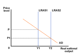
- Long-Run Equilibrium occurs where the AD curve intersects the LRAS curve. This reflects the economy’s potential output or full-employment output.
Understanding Aggregate Supply and Demand
Aggregate Supply responds to rising pricing, which motivates businesses to use more inputs to create a greater output.
The incentive is that if the price of inputs stays the same, but the price of outputs rises, the business will be able to produce and sell more, resulting in higher profits and margins.
Aggregate Supply is an upward-sloping curve and implies that a company will supply more as the price per unit rises.
In the LR, the supply curve finally turns vertical, suggesting that a business can no longer produce at a certain price due to input limitations, such as the number of employees and factories.
Aggregate Demand refers to a company's total spending, including consumer spending, investments, government spending, and net exports. The Aggregate Demand curve is a downward-sloping curve that indicates that the economy's total expenditure drops when the price level rises.
For instance, people will be spending less because rising costs have eroded their purchasing power. As outputs rise, the need for money and credit to create them rises, which leads to an increase in interest rates. However, interest rates raise fewer investments.
Furthermore, exports will fall when prices in a certain country rise, as their goods become more expensive related to other countries.
What Is Supply And Demand?
Determining the supply and demand for a good or service provides a model of price determination in a market.
The unit price of an item will fluctuate in a competitive market until it reaches a point where the quantity sought matches the quantity supplied, thus an economic equilibrium.
There are two essential laws: the Law of supply and the Law of demand.
In the long run, these two laws will influence supply and demand.
-
A shortage occurs when quantity demanded (QD) rises, but supply (S) stays unchanged, resulting in a higher price until the quantity requested is driven back to equilibrium.
-
A surplus occurs when the QD falls, but S stays unchanged, resulting in a reduced price until the QD is driven back to equilibrium.
-
A surplus arises when QD remains constant, but S increases, resulting in a reduced price until the quantity provided is driven back to equilibrium.
-
A shortage arises when QD remains constant, but S drops, resulting in a higher price until the quantity provided is driven back to equilibrium.
As a result, the market will not be in surplus or shortage when demand and supply are at the same level (known as the equilibrium point), and the market is considered efficient.
What Is The Aggregate Supply Curve?
Firms determine the supply depending on their expected earnings. Profits are defined by the price of the products a firm sells and the price of the inputs it needs to acquire, such as labor or raw materials.
-
The AS stands for total output or real GDP that businesses will generate and sell.
-
The AS curve represents the total production (real GDP) companies will create and sell at each price level.
An AS curve is seen in the graph below. The horizontal and vertical axes, the AS curve itself, and the significance of the potential GDP vertical line are the diagram's elements.
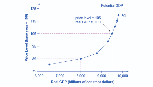
The diagram's horizontal axis represents real GDP, which is GDP corrected for inflation.
The vertical axis shows the pricing level. The average price of all products and services produced is referred to as the price level. As with the GDP deflator, it is an index number.
The price level depicted on the vertical axis is for final products or outputs purchased in the economy, not for intermediate goods and services used as inputs to production.
The AS curve depicts how suppliers respond to rising pricing for final goods and services while input prices such as labor and energy stay constant.
If enterprises confront a scenario where the price of their products or services is growing, with their production costs staying the same, the attraction of increased earnings will entice them to expand output.
What Happens If The Aggregate Supply Curve Shifts?
The AS curve has the potential to influence labor market disequilibrium or equilibrium.
There would be a supply shock if labor or another input became unexpectedly cheaper, forcing the AS curve to move outward, causing the equilibrium price to fall and the equilibrium quantity to rise:
During the SR, there is typically one fixed element of production, which is the capital. On the other hand, the fixed component has no effect on the curve's capacity to move outward.
At a given price, shifting the curve to the right generates an increase in output and a fall in GDP. A decrease in the wage rate, a rise in physical capital stock, and technical development are all examples of events that cause the SR curve to move to the right.
Because everything in the economy is considered to be utilized efficiently at this stage, only capital, labor, and technology impact the AS in the LR.
Since the LRAS curve shifts the slowest, it is typically seen as static. The LRAS curve is vertical, indicating economists' assumption that changes in AD have only a brief impact on total production.
A growth in population, an increase in physical capital stock, and technical development are all examples of events that move the LRAS curve to the right.
Why Does The Shift Occurs?
Production expenses, such as taxes, subsidies, the cost of labor (wages), and the cost of raw materials, impact the SRAS curve. When the quality and amount of labor and capital fluctuate, all of these factors cause the SR curve to alter.
Both the SRAS and LRAS curves are affected by the adjustments. Events that alter the economy's potential production impact the LRAS curve.
Changes in short-run AS lead the price level of an item or service to fall while real GDP rises. Prices stabilize in the LR, and the price level of the item or service rises in reaction to changes.
Potential GDP
The slope of the AS curve goes from almost flat on the far left to virtually vertical on the far right, as seen in the sample graph above.
The economy's production is substantially below potential GDP: the amount that an economy can create by fully using its present levels of labor, physical capital, and technology.
In the context of its market and legal institutions, at the far left of the AS curve.
Unemployment is prevalent at these low levels of output, and many factories are only operating part-time or have closed.
Because so many employees and factories are ready to swing into production, a very little increase in the prices of the outputs that firms sell, with no increase in input prices, can induce a significant jump in the amount of AS (real GDP).
However, particular organizations and industries will reach their capacity constraints when the quantity produced grows.
For example, practically all expert employees in a particular sector may have positions or factories in specific geographic locations or industries operating at maximum capacity.
A higher price level for outputs stimulates a greater amount of output in the intermediate section of the AS curve.
Nonetheless, as the AS curve's more steep upward slope demonstrates, the increase in quantity in response to a given increase in the price level will not be as substantial.
The AS curve gets almost vertical at the far right. Higher output prices could not promote extra output at this level because, even if companies seek to raise production, the economy's labor and machinery inputs are fully utilized.
The vertical axis in the illustration for the AS curve shows that potential GDP occurs at a total production of 9,500.
When an economy is working at full capacity, machinery and factories, the natural unemployment rate is quite low. As a result, potential GDP is also referred to as full-employment GDP.
Why Does The Aggregate Supply Curve Cross Potential GDP?
Typically, the AS curve is constructed to intersect the potential GDP line. How can a country's economy create more than its potential or full-employment GDP?
According to economic intuition, producers would undertake obsessive production efforts if output prices were high enough. All employees would work double overtime, and all machinery would function 24 hours a day, seven days a week.
Such hyper-intense production would go beyond completely exploiting potential labor and physical capital resources to using them in ways that are not long-term sustainable. As a result, the output can sprint over potential GDP, but only in the SR.
As a result, if demand is too low (high) in the SR, producers might deliver less (more) GDP than potential. On the other hand, producers in the LR are restricted to producing at potential GDP.
Therefore, the AS curve is also known as the SRAS curve. The LRAS curve is a vertical line that represents potential GDP.
What Is The Aggregate Demand Curve
The total expenditure on domestic goods and services in an economy is referred to as AD. In other terms, AD stands for total planned expenditure or total spending.
All four components included in AD:
-
Consumption
-
Investment
-
Government spending
-
Net exports (exports minus imports)
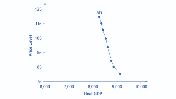
This demand is driven by a range of things, one of which is the price level. An AD curve depicts the total expenditure on domestic goods and services at each price level.
Below is an example of an AD curve. The horizontal axis represents real GDP, while the vertical axis reflects price level, just like an AS curve.
However, the curvature of the AD curve, which slopes downward, is significantly different. Increases in the price level of outputs lead to decreased overall spending, as seen by this downward curve.
So, how do price movements influence the various components of AD? The following is the formula for calculating AD:
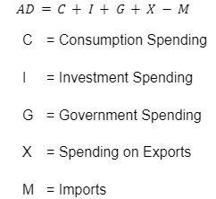
From the perspective of the wealth effect, when the price level rises, the purchasing power of savings held in bank accounts and other assets decreases as inflation gnaws away at them.
Consumer spending will decline as the price rises since a price rise diminishes people's wealth.
The interest rate impact explains why, as outputs increase, the same purchases will require more money or credit. Interest rates will rise due to the increased demand for cash and credit.
On the other hand, higher interest rates will cut company borrowing for investment and household borrowing for houses and vehicles, lowering both consumption and investment expenditure.
For example, from the perspective of the foreign pricing impact, if prices rise in the United States while being unchanged in other nations, items in the US will be proportionally more costly than commodities elsewhere.
When the price of US exports becomes more expensive, the number of exports sold will decrease. Therefore, imports from other countries will be cheaper, increasing the number of imports.
As a result, a higher domestic price level will lower net export expenditures when compared to price levels in other nations.
What Happens If The Aggregate Demand Curve Shifts?
When total consumer spending falls, the AD curve moves to the left.
Consumers may spend less because the cost of living is rising or government taxes have risen.
If consumers expect prices to grow in the future, they may decide to spend less and save more. Consumer temporal preferences may shift, and future consumption precedes current spending.
Fiscal policy that is too tight might push AD to the left. To close a budget deficit, the government may choose to raise taxes or cut spending.
Monetary policy has a more delayed impact. Individuals and corporations tend to borrow less and save more when monetary policy raises interest rates. This may cause AD to move to the left.
The fourth major variable, net exports (exports minus imports [X-M]), is less straightforward and more debatable. Changes in the capital account always balance the current account surplus.
That is a trade surplus or positive net exports. This would suggest a net inflow of foreign cash or dollars kept overseas to compensate for foreigners purchasing more US goods than they are selling to the US.
This condition would result in a rise in US foreign currency holdings or an inflow of US dollars kept overseas, boosting AD.
Why The Shift Occurs?
A variety of economic factors can influence an economy's AD.
Among the most important are:
1. Interest Rates:
Whether interest rates are rising or declining, consumer and corporate decisions will be influenced. Lower interest rates reduce the cost of financing for large-ticket items like appliances, vehicles, and properties.
Companies will also be able to borrow at lower rates, which is likely to contribute to increased capital investment. On the other hand, higher interest rates raise the cost of borrowing for both individuals and businesses.
As a result, depending on the magnitude of the rate increase, expenditure tends to fall or expand more slowly.
2. Income and Wealth:
As household wealth rises, AD tends to increase. On the other hand, a decrease in income frequently results in a reduction in AD.
Personal savings increases will also contribute to lower product demand, typical during recessions. When consumers are optimistic about the economy, they are more likely to spend, resulting in decreased savings.
3. Expectations of Inflation:
Consumers who believe that inflation or prices will grow (reduce) in the future are more likely to make purchases now, resulting in a rise (drop) in AD.
4. Currency Exchange Rates:
Foreign items will become more costly (less expensive) if the value of the US dollar decreases (rises).
Meanwhile, items made in the US will become less costly (more expensive) in international markets. As a result, the AD in the US will rise (or decrease).

Free Resources
To continue learning and advancing your career, check out these additional helpful WSO resources:


or Want to Sign up with your social account?