Law of Supply
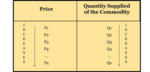
It states that the higher the price, the more prominent the quantity supplied will be, and the lower the price, the smaller the quantity supplied.


What Is the Law of Supply?
In economics, the law of supply is an important doctrine that regulates the flow of goods and services in a market.
It states that while other things remain constant, the quantity of any commodity supplied in the market is directly proportional to the price at which it sells. In other words, there will be increased supply when the prices are high and decreased when the prices are low.
The law of supply, or the 'supply hypothesis,' gives us the relationship between the price and supply of goods and services.
In other words, it states that the higher the price, the more prominent the quantity supplied will be, and the lower the price, the smaller the quantity supplied. Therefore, in terms of the supply law, the quantity supplied of a commodity is positively related to its price.
It works on the assumption of ceteris paribus, i.e., 'other things remaining the same.' The 'other things' refer to the determinants of supply other than the price of the commodity, which are listed as follows:
1. Input prices:
The supply of goods has an inverse relationship with input prices. A higher cost of inputs, such as raw materials, labor, etc., reduces the profit margin, leading to lower output by the firm at a given price. A fall in the input prices will have the opposite effect, making it profitable for the firm to produce goods.
2. Price of related goods:
In general, the supply of a commodity has an inverse relationship with the price of substitute goods.
Suppose the price of other related commodities, i.e., substitute goods, are high, and the cost of items produced by the firm remains constant. In that case, producers will find it more profitable to produce and sell the related goods. As a consequence, the supply of the current goods being produced will fall.
3. Production Technology:
Advancement in production techniques and technology reduces production costs and increases the producer's profit margin. This induces the producers to improve the product supply of the said product.
4. Nature of industry:
The supply of a commodity also depends on the nature of the industry. If the firm exists in a competitive industry, the store tends to be cut-throat due to the fear of substitution. Whereas in a monopoly, the firm has greater control over supply.
5. The policy of taxation and subsidies:
The imposition of indirect taxes like excise duty, sales tax, GST, etc., increases the cost of production and thus decreases the supply of the good. On the other hand, government subsidies on producing goods will reduce costs and induce firms to increase the supply.
6. Expectations about future prices:
If the producers expect that the prices of a particular good will increase shortly, they will reduce the current supply and offer large quantities of the goods at high prices to earn higher profits.
Conversely, expectations of a fall in future prices tend to increase supply in the present period.
7. Natural factors:
Natural factors like drought, flood, unfavorable climatic conditions, etc., adversely affect the supply of some commodities. Heavy rains, floods, and drought conditions lead to a decrease in the collection of perishable goods.
The law of supply assumes that these determinants of supply do not change. The supply law can be illustrated with the help of a supply schedule and supply curve that we will see in the coming sections.
Key Takeways
- The law of supply states that while other things remain the same, the quantity of any commodity supplied in the market is directly proportional to the price at which it sells.
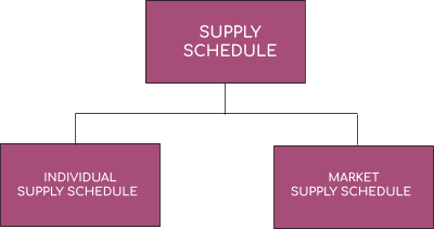
- A supply schedule is a tabular statement showing various quantities producers are willing to produce and sell at various prices during a given period. It is of two types:
- Individual supply schedule, i.e., supply schedule of an individual seller.
- Market supply schedule, i.e., the supply schedule of all the firms in the market.
- A supply curve is defined as a curve that shows various quantities of a commodity that producers are willing to produce and sell at different prices during a given period. It is of two types:
- Individual supply curve, i.e., the supply curve for an individual seller.
- Market supply curve, i.e., the supply curve for all the sellers in the market.
- The positive slope of the supply curve works on three factors:
- The higher the price, the higher the profits.
- Increase in the marginal cost of production.
- Increase in prospective sellers with an increase in prices.
- There are three types of supply based on time:
- Market period - a very short period where the supply is fixed and cannot be changed, as in the case of perishable goods.
- Short run period - a short period where supply can be changed to some extent.
- Long run period - a long period where the quantity supplied can be changed completely.
- A supply curve is normally positively sloping; however, the following are the exceptions in certain cases:
- The vertical supply curve in the case of supply goods such as rare paintings, vintage cars, etc.
- The backward-sloping supply curve, as in the case of the supply of workers and their respective wages.
Understanding the Law Of Supply
An economic theory known as the law of supply forecasts how the cost of products and services will impact their availability. It states that firms will expand the range of products and services they offer when prices grow.
Despite its applicability in economic decision-making, the law of supply ignores other variables that may impact supply, such as shifts in production costs and the level of competition.
However, knowing the law of supply, its exceptions, and other pertinent information can help businesses decide how much to charge for their goods and services and how to modify their supply in order to maximize profits.
In actuality, the connection between supply and demand frequently determines prices. The law of supply and demand, a related economic theory, explains how this operates. Prices typically rise in response to increased demand for goods and services.
This incentivizes providers to enhance their supply. But fewer people will purchase those goods and services as long as their costs keep rising.
Therefore, open markets are expected to progress towards an equilibrium point where the amount and price of supply precisely meet the demand of customers, according to the law of supply and demand.
Exceptions to the Law of Supply
The supply curve generally slopes upward and to the right, but it may take a different shape in some exceptional circumstances. It is significant to observe the two unique forms of the supply curve.
1. Vertical Supply Curve:
There are certain commodities, the supply of which cannot be increased or decreased at all. Thus, the collection is fixed in the case of rare goods such as classical paintings, old manuscripts, rare postage stamps, old coins, etc.
In some other cases, the supply may be fixed in the short run and can only be increased in the long run. As stated in the example of wheat and other agricultural products, the supply is fixed once the crop is grown and can be increased only in the long run.
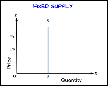
In such cases, the supply curve will be a vertical line parallel to the OY, as illustrated in the above picture.
2. Backward Sloping Supply Curve:
Sometimes, a part of the supply curve may have a backward slope. This would mean that a smaller quantity would be offered at a higher price than a lower price.
This type of backward-sloping supply curve may occur in the labor supply, wherein the store is expressed in the number of hours worked.
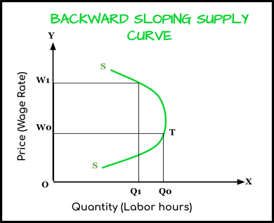
As demonstrated in the above picture, when the wage is OW, the labor supply is OQ; but when the wage rate rises to OW1, the collection falls to OQ1. As a result, the supply curve SS has a negative slope beyond point T.
As the wage rate (the price of labor) increases, workers work more hours initially to earn more income. The workers here may prefer delivery to leisure.
The worker may be willing to work for fewer hours at a very high wage rate to enjoy more leisure. At a very high wage rate, the worker prefers peace to work as he may have earned enough income to satisfy himself.
What is a Supply Schedule?
A supply schedule is a tabular statement that shows various quantities of goods the producers are willing to produce and sell at multiple alternative prices during a given period.
Supply schedules are of two types:
- Individual Supply Schedule
- Market Supply Schedule
1. Individual Supply Schedule:
An individual supply schedule is a table that shows various quantities of a commodity at which a particular supplier is willing to produce and sell at different prices during a given period, assuming that other factors remain the same.
For example, Bob, a producer, is willing to sell 5000 kg of a commodity X when its price is $10 per kg. If the price increases to $15 per kg, he is willing to sell 10,000 kg of commodity X.
Below is a supply schedule of how much Bob is willing to sell at prices: $10, $15, $20, $25, and $30 per kg.
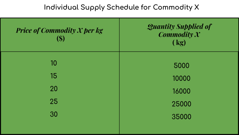
As seen in the supply schedule above, when the price is $10 per kg, the supply is 5000 kg. When the price increases to $15 per kg, the collection also increases by 10,000 kilograms. With every rise in the price of commodity X, the quantity also supplied increases. At $30 per kg, the amount given is 35000 kg.
2. Market Supply Schedule:
The market supply schedule is the table that shows various quantities of a commodity on which all the firms or producers are willing to supply at each given market price during a specific period assuming other things remain the same.
A market supply schedule is the summation of all the individual supply schedules.
For example, when the price of commodity X is $10 per kg, producers are willing to supply 9,000 kilograms per week. At $20 per kg, the quantity supplied is 36,000 kg per week. As the given market price has increased, so has the supply of commodities.
Given below is the market supply schedule of the same.
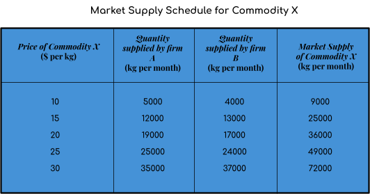
The schedule precisely demonstrates the application of the law of supply. In other words, it is the tabular presentation of the law of supply.
What is a Supply Curve?
A supply curve is a graphical representation of the law of supply. It conveys the same information as a supply schedule but diagrammatically.
Like the supply schedule, the supply curve is also of two types:
- Individual Supply Curve
- Market Supply Curve
1. Individual Supply Curve:
An individual supply curve is defined as the curve that shows various quantities of a given commodity that a particular producer is willing to supply at different prices during a given period, assuming no change in other factors of the item.
Below is the supply curve for commodity X, based on the individual supply schedule mentioned above.
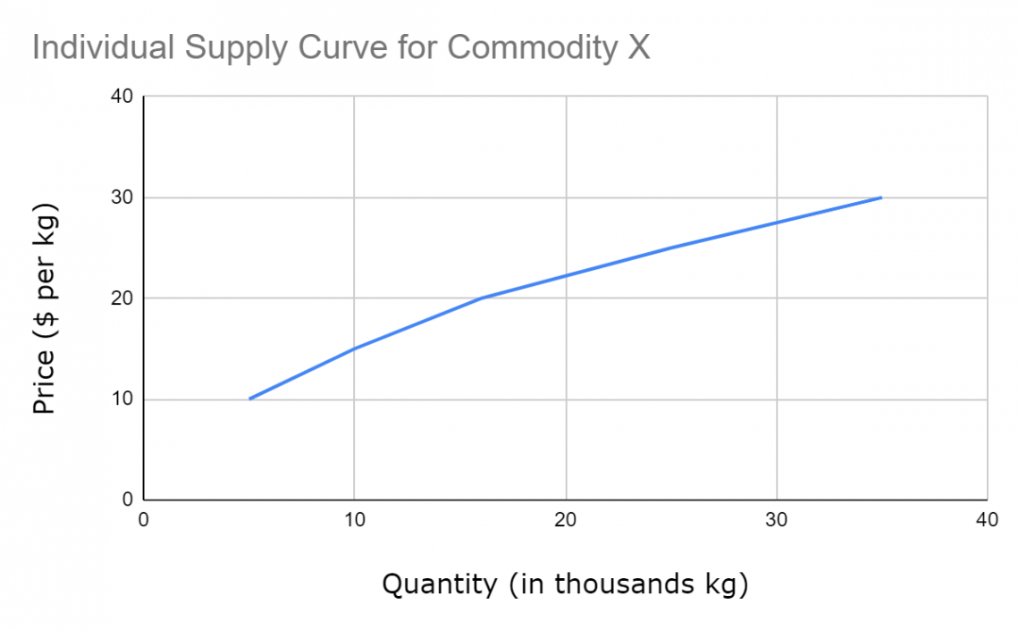
The positively sloping supply curve shows the direct relationship between the price and the quantity supplied.
2. Market Supply Curve:
A market supply curve is a curve that shows various quantities of a commodity that all the producers are willing to produce and sell at different prices during a given period, assuming that there is no change in the other factors of the commodity.
Given below is the market supply curve of commodity X based on the market supply schedule above.
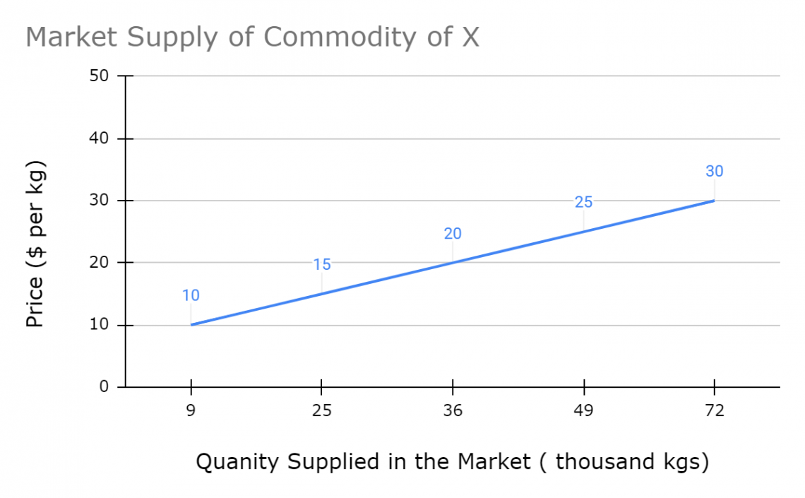
A market supply curve is usually an upward (positive) sloping curve from left to right, indicating a direct relationship between price and supply. A market supply curve is sometimes called an Industry supply curve.
Explaining the Supply Hypothesis
The supply hypothesis, or the law of supply, demonstrates a positive relationship between the commodity's price and the quantity supplied. A positively sloping supply curve indicates the same.
The positive slope of a supply curve can be explained in terms of three factors:
1. Higher the price, higher the profits:
The level of price of a commodity determines the profits it generates. The higher the cost of the item, the greater the profit; ceteris paribus (i.e., other things remaining the same). This high price then incentivizes the manufacturer to produce and sell more significant goods.
2. Increase in the Marginal Cost of Production:
The marginal cost of production is the change in the total production cost due to the production of one extra unit. It works on the principles of the law of diminishing returns.
In most cases, the marginal cost of production increases with increased production units. The producers would be willing to produce and supply a larger quantity of the commodity only at a higher price to cover the marginal cost of production.
When the marginal cost exceeds the expected profit, the product is no longer attractive to the manufacturer.
3. Increase in prospective sellers with the increase in prices:
A price rise will give incentive not only to the existing producers of a commodity but will also motivate the other future producers to produce the commodity to earn higher profits.
For example, a rise in the price of rice will motivate farmers to produce more rice instead of other goods, like wheat. The farmers will withdraw resources from grain production and devote the same to rice production.
Thus, more firms are willing to enter the market to produce the goods at higher prices.
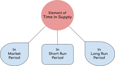
4. Element of Time in Supply:
Economists distinguish between different types of supply curves based on how supply responds to a change in price in terms of the time element. We may divide time into the following three periods based on supply and response to a change in price:
- Market Period
- Short-Run Period
- Long-Run
1. Market Period:
The market period is a brief period in which the supply is fixed. The entire collection in the market period is the stock that has already been produced.
For example, in the case of the supply of perishable goods, once the vegetables have been grown and brought to the market, there cannot be any change in the collection of vegetables, no matter the price.
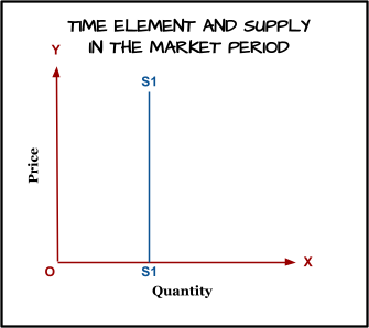
Thus, in the market period, firms cannot adjust their output to any change in price. As a result, the supply curve of a firm or an industry is vertical, as illustrated by the supply curve S1S1 in the above picture.
2. Short-Run:
The short run is the period in which the supply can be adjusted. Producers can increase production by running the existing plant for longer hours, like running a show for two shifts instead of one.
The short-run period is not long enough for firms to set up a new plant or machinery. Therefore, in the short run, supply can be increased to a limited extent.
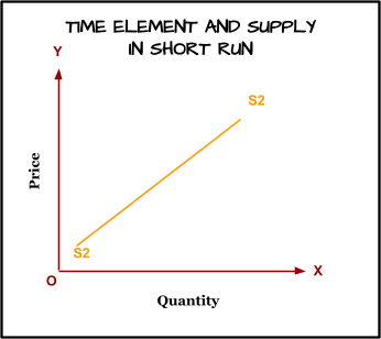
For example, a bag manufacturer can increase his supply to a limit by making workers work 2 hours extra each day. So if 120 bags were produced in a day by working 8 hours earlier, after increasing the working hours by 2 hours, the supply would increase to 150 bags per day.
The short-run supply curve is upward-sloping, as illustrated by the S2S2 above.
3. Long-Run:
In the long run, the firms can build new plants or close down the old ones. Moreover, new firms can enter the industry and set up new plants making it possible to bring about a massive change in the quantity supplied of a commodity in the long run.
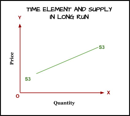
Take the example of the same bag manufacturer with one plant that manufactured 120 bags in 8 hours. If the bag manufacturer adds two more plants in the long run, it can increase its supply to 360 bags in 8 hours, i.e., triple its collection in the coming future by increasing its production capacity.
A flatter supply curve, S3S3, illustrates this in the above pic.


or Want to Sign up with your social account?