Option Pricing Models
Option Pricing Models are frameworks that help derive a fair value for options.


What Are Option Pricing Models?
Option Pricing Models are mathematical models that use several variables to develop an option’s fair, theoretical value.
If we knew where the market would be at the expiration date of an option, we would price options perfectly. However, we do not know this and hence need option pricing models based on probability theory.
These are beneficial as they help measure and price the risk associated with options, they are useful when evaluating exposure to price fluctuations, they provide a benchmark for options to promote fair trading, and some models allow for a wide variety of scenarios to be accounted for.
However, extreme market events may render these models ineffective, so one must take care when assessing assumptions vs reality. Providing accurate inputs into these models can be difficult since many are estimates.
- Option Pricing Models are frameworks that help derive a fair value for options.
- Options are assets that derive their value from other assets, and their cash flows depend on the occurrence of specific events.
- The option value is determined by the forces of demand and supply of the option.
- Different economic factors affect calls and put values differently.
- There are three main options for pricing: Black-Scholes, Binomial option pricing, and Monte-Carlo simulation.
Understanding The Option Pricing Theory
Generally, the value of an asset is derived by looking at the present value of future cash flows that the asset will generate. However, other assets derive their value from the value of another asset, and the asset’s cash flows are contingent on the occurrence of specific events. These are called options.
An option provides the holder the right to buy or sell a specified asset quantity at the strike price (fixed price). The strike price or fixed price is a price that was agreed upon when the option contract was made, on or before the option’s expiration date.
Since it is a right and not an obligation, the holder can buy it, sell it, or allow it to expire. The two types of options are: call options and put options.
Types of Options
There are two types of options - call options and put options. Below, we will explore each type, focusing on what they mean, how to calculate each option's gross and net profit, and how they each derive their net payoff according to the strike price.
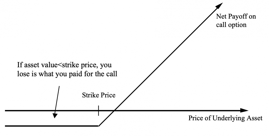
A call option gives the buyer of the option the right to purchase the underlying asset at a strike price before the expiration date.
If, on the expiration date, the value of the asset is less than the strike price, the option is worthless and not exercised. However, if the asset’s value is higher than the strike price on the expiration date, the option is exercised, and the buyer obtains it at the strike price.
We can then say that
Gross Profit = Value of asset on expiration date - Strike Price
Also, we can say that
Net Profit = Gross Profit - Price paid for the call initially
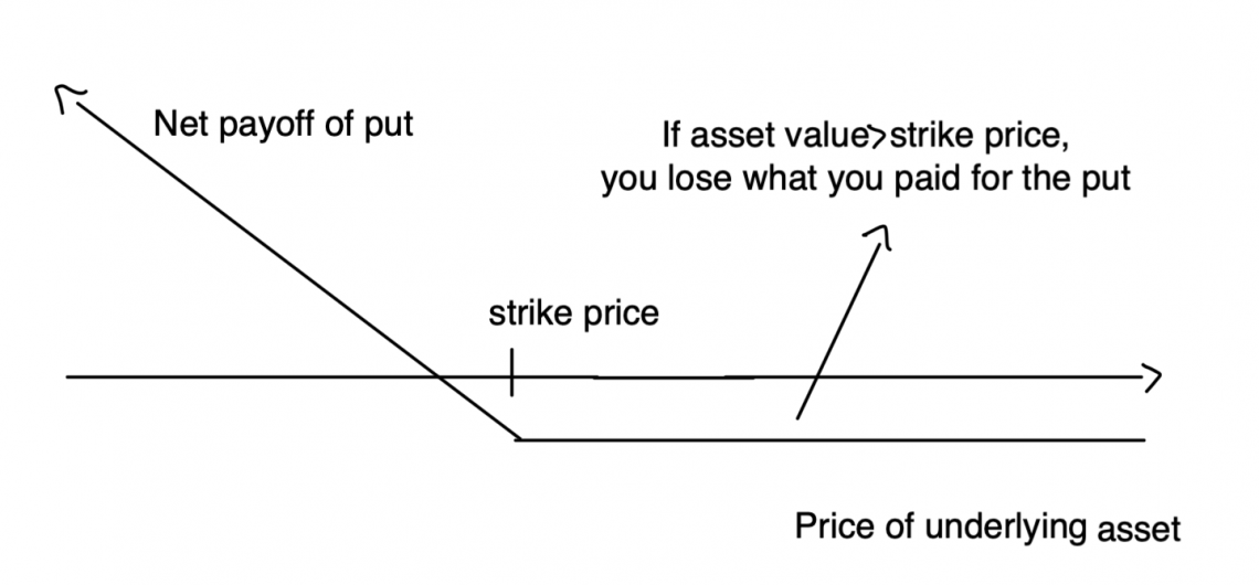
A put option gives the buyer of the option the right to sell the underlying asset at a strike price, on or before the expiration date.
If, on the expiration date, the value of the asset is higher than the strike price, the option will not be exercised and will expire worthless. However, if the asset’s value on the expiration date is lower than the strike price, the buyer will sell the asset at the strike price.
We can then say that
Gross Profit = Strike Price - Market Value of the Asset
We can also infer that
Net Profit = Gross Profit - Price paid for the option initially

Example of Call and Put Options
Let us look at the example of Call and Put Options:
Call option: suppose we buy 100 shares
- Price initially paid for option = $3 per share
- Strike price = $50
- Market of share at expiration = $100
So,
Gross profit = (100 * 100) - (100 * 50) = $5,000
Net profit = $5,000 - (100 * $3) = $4,700
Put option:
- Price initially paid for option = $5
- Strike price = $100
- Value of asset at expiration = $90
The buyer of the option sells the asset at the strike price and buys it back at the expiration value:
Gross profit = $100 - $90 = $10
Net profit = $10 - $5 = $5
Determinants of Option Value
The table below is a snapshot of how the Call value and Put value can change with different factors. It is worth noting that the Call value and Put value change differently with each factor:
| Factor | Call Value | Put Value |
|---|---|---|
| Increase in underlying asset value | Increase | Decrease |
| Increase in strike price | Decrease | Increase |
| Increase in variance of asset value | Increase | Increase |
| Increase in time to expiration | Increase | Increase |
| Increase in interest rate | Increase | Decrease |
| Increase in dividends paid | Decrease | Increase |
Types of Option Pricing Models
Several models are used in Option Pricing. Some methods are more realistic than others, some contain more assumptions, and some are used for specific options (American or European).
While an analyst may want to use a specific model of their choice, they may be restricted to a certain model depending on the information available to them. This is evident from the various factors each formula needs for each model, as we will see below.
Black-Scholes Model
This is a method used to price European options.
It includes certain assumptions including:
- No dividends are paid out
- Interest rate is constant
- No taxes
- Stock is perfectly liquid
- Option can only be exercised at maturity (European option)
Black-Scholes formula:
Put options → P = Xe − rTΦ(−d2) − S0Φ(−d1)
Call options → C = S0Φ(d1) − Xe − rTΦ(d2)
Where
- X = Strike price
- S0 = Current stock price
- R = risk-free interest rate
- T = time to expiration (in years)
- Φ = cumulative distributive function
d1 = (ln(S0/X) + (r + (σ²/2))/(σ√T)
d2 = d1 - σ√T
Binomial Model
In the binomial model, we consider valuing an asset by a process in which, at any time period, the asset can move to any two prices.
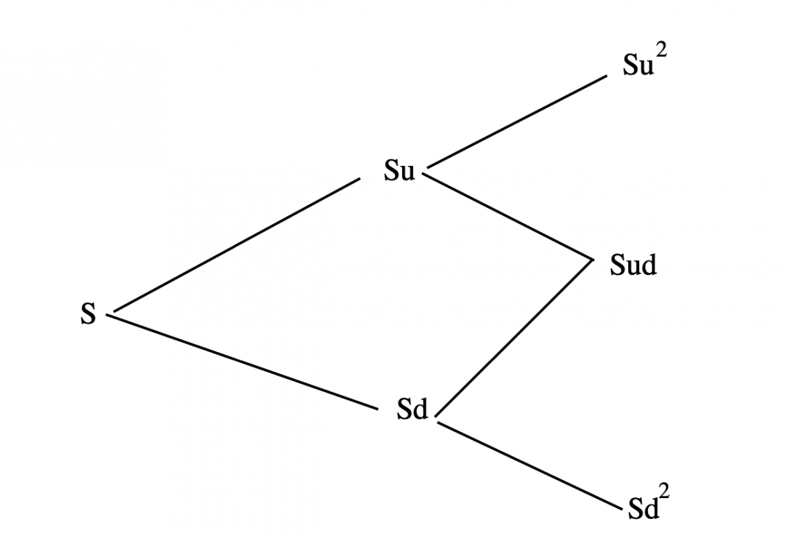
In the diagram above, S is the current stock price; this price can move up to Su with probability p or move down to Sd with probability 1-p.
To determine how many units of the asset to buy, we can use the general formula:
Δ = Number of units of the underlying asset bought = (Cu - Cd)/ (Su - Sd)
Where:
- Cu = value of call if the stock price is Su
- Cd = value of call if the stock price is Sd
Note
This process is iterative if repeated for several time periods.
Value of the call = (Current value of the underlying asset * Number of units of the underlying asset bought) - Borrowing needed to replicate the option
Monte-Carlo Simulation
This is a valuation method used to predict the probabilities of a variety of outcomes when the potential for random variables is present. In this method, we aim to aggregate several different outcomes many times and find the probabilities of different option values.
Using the binomial model, we consider what would happen when the asset price goes up or down by determining the growth shocks in the asset price. We can calculate this from the following formula when the asset price goes up or down, respectively:
If the asset price goes up → û = e(r - δ - 0.5σ² )h + σ√h
If the asset price goes down → dࠦ = e(r - δ - 0.5σ² )h - σ√h
- h = T/N, where N is the number of periods calculated
- h = length of a period
After we have found expected payoffs for the desired future time periods, we apply a discount rate to these to obtain a value in today’s terms.
On the other hand, in continuous time, we would have an infinite amount of time periods between two points in the future.
Therefore, we would have to use the Geometric Brownian Motion (GBM), which implies that the asset follows a random walk. A random walk suggests that historical patterns cannot determine future asset prices because price changes are independent of each other.
To calculate the change in a stock (asset) price, we can utilize the following formula:
ΔS = S (μΔt + σε√Δt)

Where:
- S = current stock price
- μ = expected return
- t = time
- σ = standard deviation of stock returns
For continuous time periods, we do not need to calculate the value of the stock (asset) at every period, only at maturity. This can be done with the following formula:
S(T) = S0e((r - δ - 0.5σ² )T + σε√T)
Once again when we find expected values, we discount them to obtain a value in today’s terms.
Option Pricing Model FAQs
European options can only be exercised at the expiration date. American options can be exercised before or on the expiration date.
Primarily, there are two types:
- Call options give the holder the right to buy an asset at the strike price, on or before the expiration date
- Put options give the holder the right to sell an asset at the strike price, on or before the expiration date
The three models are:
- Black-Scholes - used for European options
- Binomial Option Pricing - uses a tree method to represent possible price movements of the underlying asset at discrete time intervals until expiration.
- Monte-Carlo simulation - uses random sampling to simulate the price paths of the underlying asset.
There is no Option Pricing Model that is classified as the best. Different models will need to be used depending on the data available to input. However, the Binomial Model is most popular for American stocks.
Buyers and sellers set the prices of options. There is no single entity who determines the price of an option. Prices of options follow the same laws of demand and supply in a market.
Free Resources
To continue learning and advancing your career, check out these additional helpful WSO resources:


or Want to Sign up with your social account?