AVERAGEIF Function

What is the AVERAGEIF Function?

The AVERAGEIF function in Excel is a statistical function that calculates the average (arithmetic mean) of a range of cells that meet specific criteria.

In school, work, or life, you may have heard of finding the average to something we deal with or with something we want to know. For example, a school teacher may say the average grade people received in class was 80%. Financial analysts also use the average to find the average in their jobs. 

You could have also heard the average height of men or women. When you hear of this, consider it the standard or the typical. Typically doctors use the average for the height of people. 

It is used financially to find the average home cost in a town or city. It is used in the medical and scientific fields to determine how much people sleep on average. But, as you see, the average can be applied to many things in life and all around you. 

Finding Averages

You may ask yourself, well, how can we find the average? Before getting into the function of Excel, knowing your basics is essential. Now that you know where and how it can be applied, we can proceed to how we find it.

If you want to calculate the average, add all your values together. For example, by adding the numbers 2,7,10,4,6 and 1. Then proceed to find the total numbers:

2 + 7 + 10 + 4 + 6 + 1 = 30. 

Our total from the numbers we added was thirty. Now you will divide the thirty by the number of numbers you initially added. In this case, we added a total of six numbers. 

After dividing thirty by six, our final result is five. This is our average. So to find the average, you need your total and divide it by the amount you added together, and your result will be averaged. 

The average can also be described as the mean. The mean is finding the average. It is mostly in grade school where the mean is used. It is also used along with the mode and median. 

The mode, median, and median are all measured in simple terms in the middle range of the data.

The formula for The AVERAGEIF Function

When using the function in Excel, the formula will be as follows:

AVERAGEIF(range, criteria, [average_range])

This is an example of how it appears in Excel when you are getting ready to enter it. 

Knowing what each of these arguments means and what they ask of is essential. If something is entered that the argument does not allow, the average will not calculate it, and it can result in an error. 

• Range - this entry can include any data containing numbers, names, or even references containing numbers. 
• Criteria - This argument can contain a number, words to interpret which cell is averaged, or expressions. For example, 64, "64", >64, oranges, or cell names such as A5.
• Average_range - is the cell on Excel that is to be averaged. 

The arguments range and criteria are required. The average range is optional, although if you do not choose to enter the average range, the range will be used. 

Things to consider

There are some things to consider when using the formula. 

• If any of your cells from the range argument are true or false, these cells will be examined. 
• If you choose to use average_range and one of the cells in the data is empty, the AVERAGEIF function will ignore it. 
• When entering the criteria entry, if there is an empty cell, it will be counted as a zero.
• Always start your formula with an equal sign. If not, the formula will not calculate.
• For the criteria argument, if you are using a name or greater than or less than sign, you need to start it with double quotation marks at the beginning and end if you are typing it. 

Examples of AVERAGEIF Function

Now that we know about the formula, let's put it into practice. 

Example #1

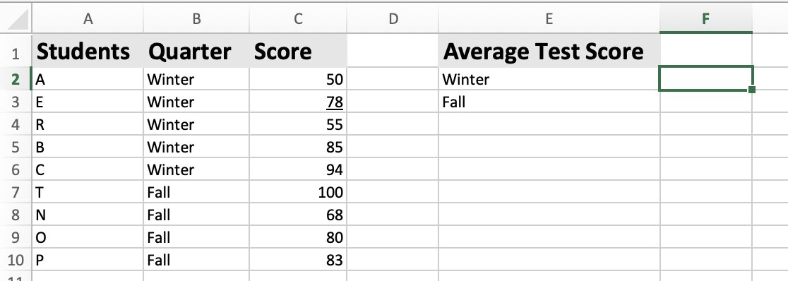
We are teachers and want to find our students' average scores in the following quarters. Our data will be as shown below.

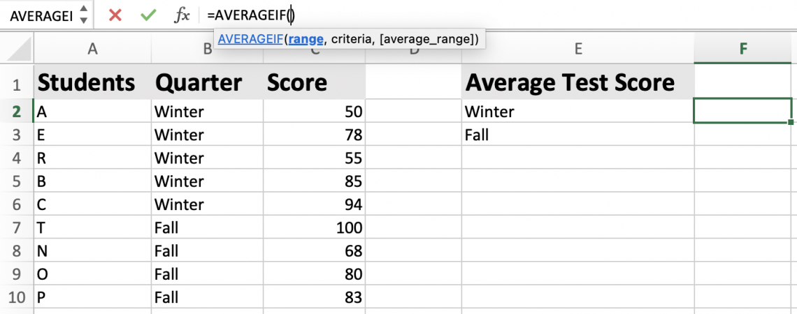
Once your data is set up, you will select the cell where your formula will be calculated. Once you select the desired cell, you will proceed to enter the formula. For the example, we will calculate the AVERAGEIF of winter first. 

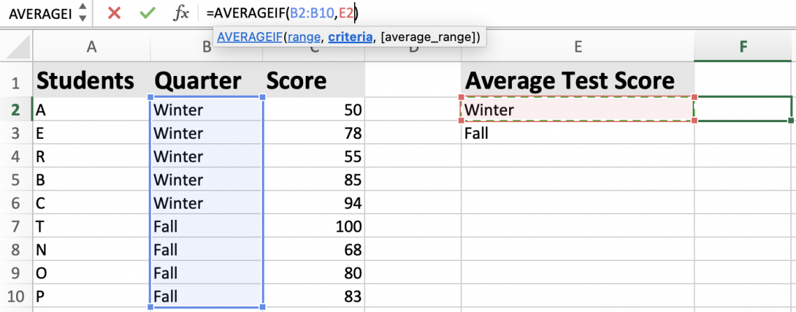
Notice how we have selected the cell F2 to be where we want our formula to be calculated. The first entry you will enter will be the range. For the range, we will enter the quarter season.

In the example above, we have selected our entire range. When entering the range, you can type it manually or select all the cells you wish to have entered. In the example, we selected the cells, which is why the cell names are in the range argument. 

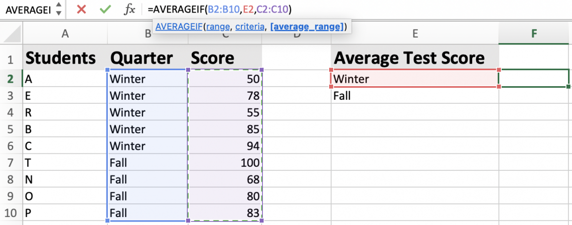
Now we will proceed with the second argument. For our second argument, we will enter the criteria, i.e., what quarter we are looking for specifically from our range. 

Again for this entry, we selected the cell we wish to enter for our criteria argument. 

The last entry will be the average range. For our average range, we will select the scores. 

After entering the average range, we will have completed all the formula's arguments. Then, in our next step, we press enter so that our formula calculates and we get our result. 

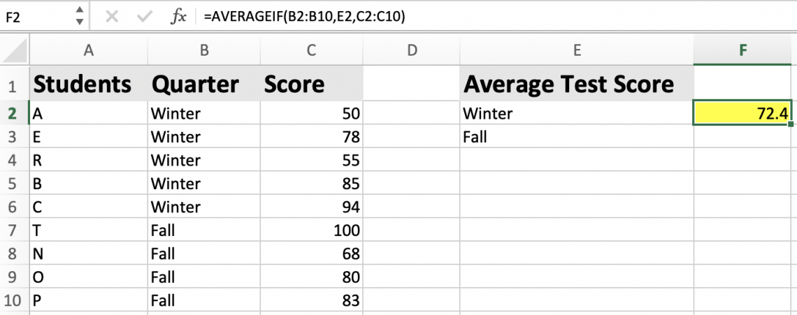
As we see, our average for the winter will be seventy-two point four. 

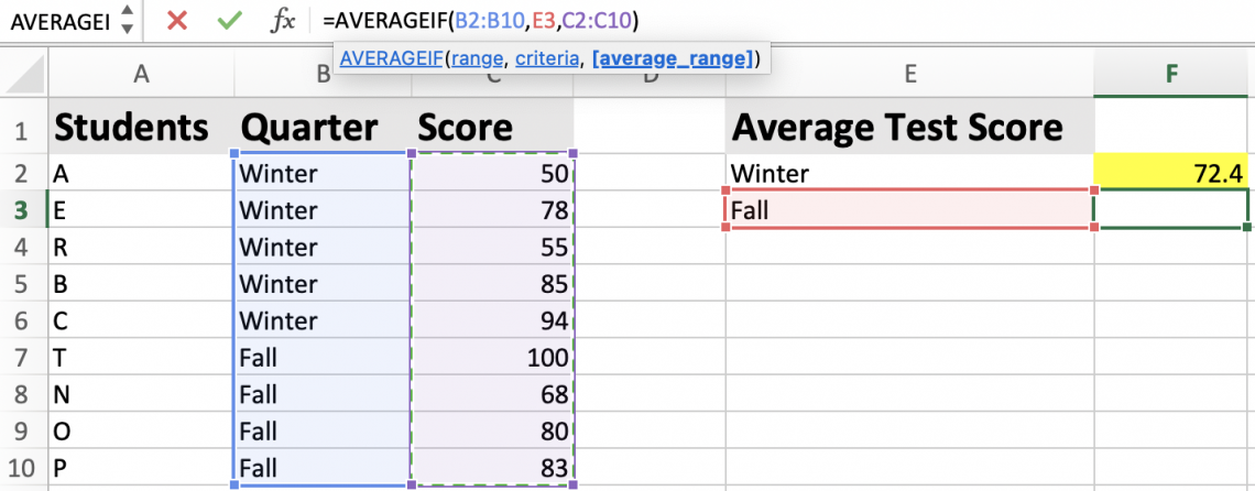
We then calculate the fall using the same method as above. However, now our criteria will change from winter to fall. After entering all the needed data, select enter to see the result. 

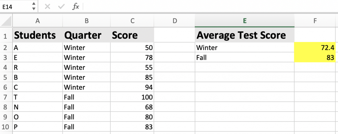
Our winter and fall results are different. The average fall score is eighty-three, and the winter score is seventy-two point four. 

Example #2 

For the following example, we will find the average sales, not the average range. The data will be as shown.

It is almost the same setup as our previous example. This example has different data. Therefore, we will proceed by selecting again the cell where we want our result and begin entering the formula. 

For this example, our range will be our sales. As you can see, we selected the cells we wanted in our range argument. To go to the following argument, we type a comma. 

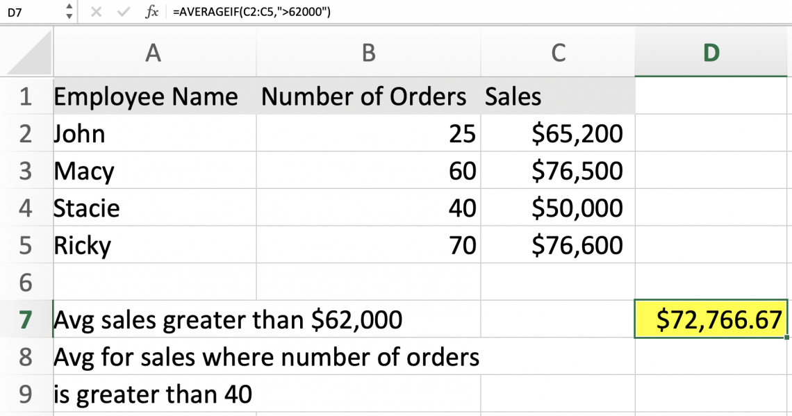
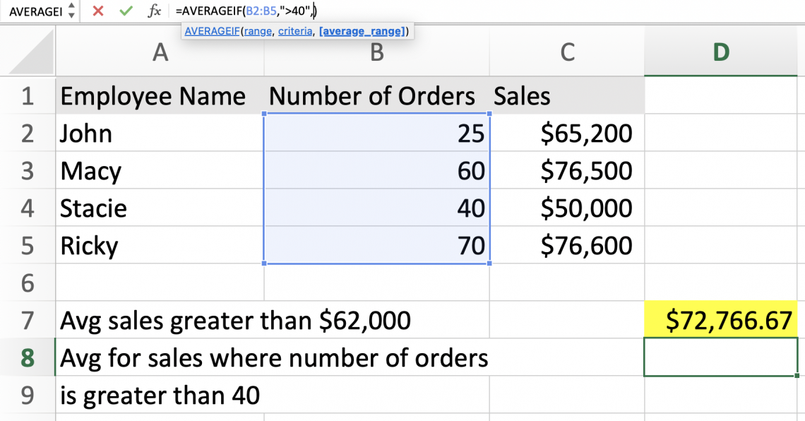
The criteria we want here is sales greater than $62,000. For this, we will type it in as ">62000." Notice how we do not enter a comma in sixty-two thousand because if we do, it will mean that we want to move on to the following argument in the formula. 

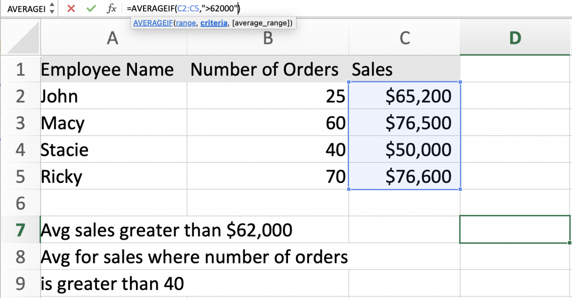
Once we have our entry, we will not enter the average range argument. Remember that the average range is optional. The function will use the range when you choose not to enter it. In this case, our sales. 

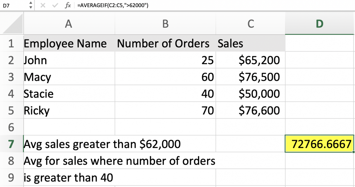
As you can see, our number came out outside of currency form. To change, right-click or double-tap your mouse pad and select format cells. 

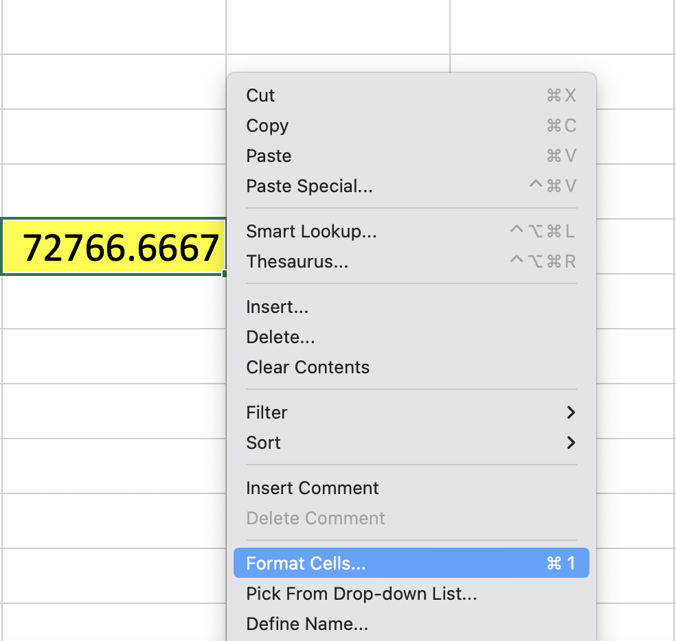
After selecting "Format Cells…," select the currency option and adjust the decimal place to two. 

Our final result will then be in the correct form.

Now let's calculate the average sales with orders greater than 40. We select the cell we want our result in and select our range. Here our range will be the number of orders. 

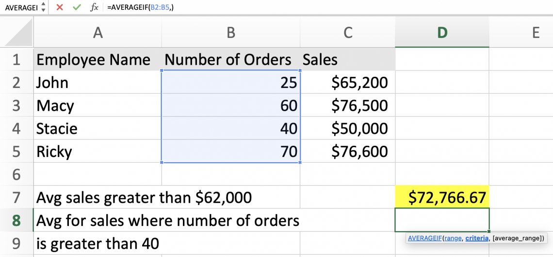
Now we will enter our criteria. Our criteria will be the orders greater than 40, which will be entered as shown below. 

We will then use the average range to select what we want to have averaged, which will be our sales. 

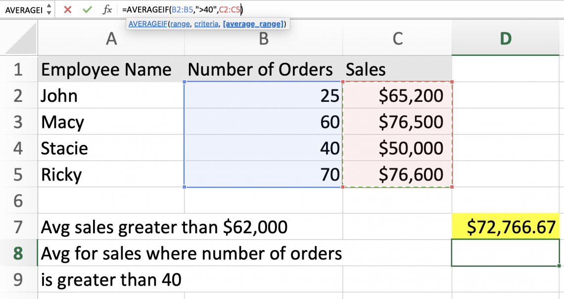
Before selecting, enter your data like the above image. Then once you are ready, you press enter to get the result. 

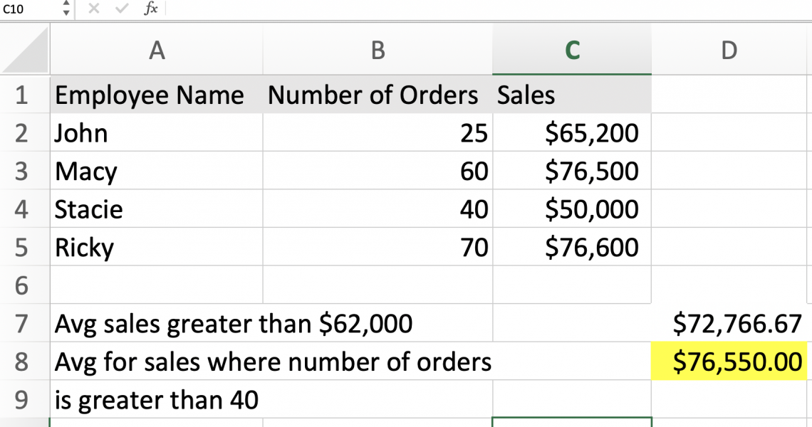
We have now found the average using the function AVERAGEIF for sales greater than $62,000 and for sales with a number of orders greater than 40.

Conclusion

Excel's AVERAGEIF function is a dynamic tool for figuring out averages depending on predefined parameters. Its adaptability to various data types and settings is what gives it its versatility; it gives customers a thorough way to efficiently analyze their datasets.

Through comprehension of its dimensions and formula structure, individuals from many sectors might obtain significant insights to support their decision-making procedures.

AVERAGEIF is a dependable technique for identifying key tendencies inside datasets, whether examining scientific data for research, financial trends in business, or student achievement in education.

Professionals looking to extract meaningful insights from their data will find it an invaluable tool due to its accurate computations and ability to handle a wide variety of data formats.

AVERAGEIF gives users the ability to easily browse complicated datasets and find trends, patterns, and outliers that drive informed decision-making and strategic planning.

Free Resources

To continue learning and advancing your career, check out these additional helpful WSO resources:

• CELL Function
• COUNT Function
• F.INV.RT Function
• ISODD Function
• MROUND Function