COVAR Function
Function in Excel calculates the covariance between two data sets, measuring their degree of joint variability

What is the COVAR Function?
The COVAR function in Excel calculates the covariance between two data sets, measuring their degree of joint variability. Covariance is a statistical measure that quantifies the degree to which two variables change together.
Covariance explains how two variables are related to each other and whether they increase or decrease simultaneously. While covariance can be applied across various fields, finance is one of its most important uses.
Portfolio Managers have a duty to their clients to build out investments that minimize risk and maximize returns; reducing risk is where covariance comes in.
It determines the degree to which two asset classes in a portfolio change together, giving a clearer picture of whether one asset’s returns depend on the other.
To illustrate, if a portfolio manager invests in stocks and bonds, it is important to understand how these two asset classes correlate during market volatility and whether they move in opposite or similar directions.
Based on this information, the bond weights can be reassigned to mitigate the risk posed by stocks. Another application would be the estimation of beta, a measurement that compares the volatility of a security or portfolio concerning the entire market.
Key Takeaways
- The COVAR function in Excel calculates covariance, measuring joint variability between two datasets. This function is crucial for minimizing risk and optimizing returns in portfolio management.
- COVAR requires mean values and deviations to compute covariance. This provides insight into how asset classes within a portfolio move together, aiding in risk assessment and allocation adjustments.
- Employing the COVAR function involves selecting the arrays of variables for calculation, simplifying the process compared to manual computation, but it assumes a sample covariance by default.
- Covariance values indicate the degree of relationship between variables, with positive, negative, or zero covariance signifying simultaneous increase, decrease, or lack of linear relationship, respectively.
Covariance Formula
Various components are required to calculate covariance, namely the mean of both variables and the deviation of individual values of a variable from its mean.
The formula can be represented in the following manner:
Covariance (X, Y) = [Σ(Xi - Xbar) * (Yi - Ybar)]/ n -1
Where
- Xi and Yi: Individual values of variables X and Y
- Xbar and Ybar: The mean of X and Y
- Σ: Sum of values for (Xi - Xbar) * (Yi - Ybar)
- n: Sample size of the dataset
COVAR Function Formula
An additional method to calculate covariance would be the COVAR function in Excel. It can be found in the Formulas tab under compatibility functions; when used, the COVAR function in Excel delivers the sample covariance by default.
The syntax can be expressed as
=COVAR(x, y)
where
- x is a selection of all variable x observations
- y is an array of variable y values
For example, if the x variable data is in cells A1:A10 and the y variable values are located in cells B1:B10, the COVAR syntax would be written as:
=COVAR(A1:A10, B1:B10)
Note
There are different variations of this function known as COVARIANCE.P (returns the covariance for an entire population) and COVARIANCE.S (provides the covariance for a sample).
Example of Covariance Calculation
To demonstrate how covariance is broken down, an example of monthly returns for Verizon (VZ) and the S&P 500 is taken. A table with the recorded returns is displayed below:
| Month | Verizon (VZ) Monthly Returns | S&P 500 Monthly Returns |
|---|---|---|
| Jan | -5.74% | -1.11% |
| Feb | 1.00% | 2.61% |
| March | 5.15% | 4.24% |
| April | 0.46% | 5.24% |
(Data Source: SH3 FactSet VZ Data, SH3 FactSet S&P 500 Data)
Step 1
Take the average returns for each variable over the four months listed above.
The average for VZ monthly returns is 0.22%, as observed using the AVERAGE function on
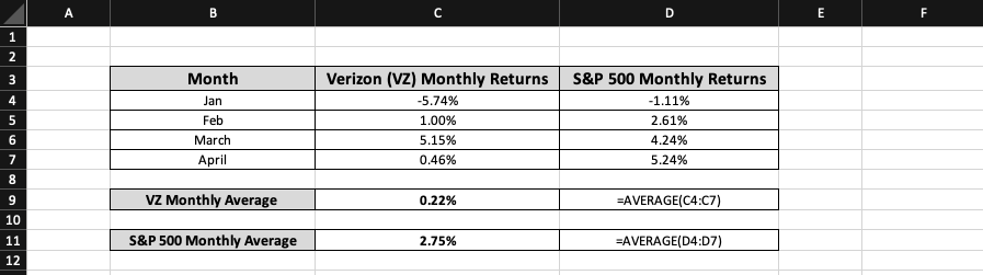
Verizon cells C4:C7, while the S&P 500 monthly return average is shown as 2.75% by taking the mean of cells D4:D7. This is the initial component of the covariance calculation.
Step 2
Subtract each observation from the corresponding monthly return average.
The covariance formula depicts this step in the numerator as (Xi - Xbar) * (Yi - Ybar). To begin, one must subtract the January observation of VZ from the VZ monthly return average.
Once complete, the following step should be replicated for the S&P 500 before multiplying both values to give the January result (Xi - Xbar) * (Yi - Ybar).
A summarization of the entire procedure is provided below for all four months:
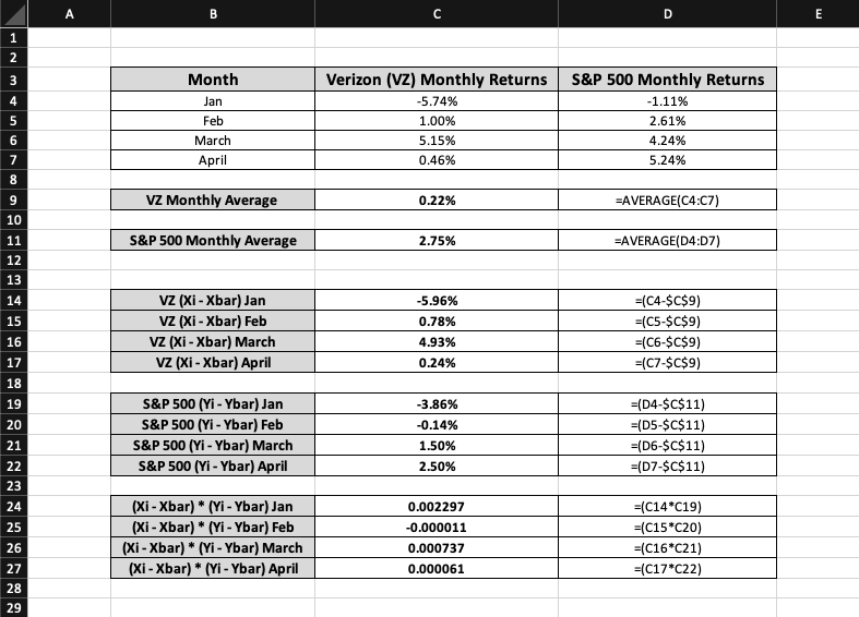
There are a few rules one must follow for these calculations. The average for variables should have dollar signs since that number is fixed while the individual observations for each month keep changing.
Additionally, converting the final (Xi - Xbar) * (Yi - Ybar) values from percentage to number is important because covariance is never expressed as a percentage.
Step 3
Summation of (Xi - Xbar) * (Yi - Ybar) values for each month.
This requires adding all the final outputs from the previous step; the resulting number represents the covariance numerator. Its calculation is provided below:
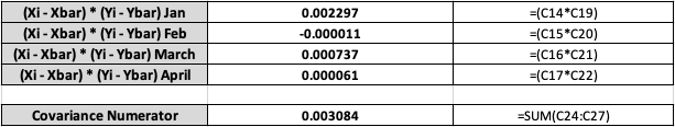
The sum of all (Xi - Xbar) * (Yi - Ybar) monthly observations is 0.003084; this can be rounded off to produce a covariance numerator of roughly 0.0031.
Step 4
Divide Covariance Numerator by (n - 1)
To conclude, the covariance numerator is divided by its denominator, which is represented as (n-1). Since the data contain four months, the covariance denominator would be 4 - 1 = 3.
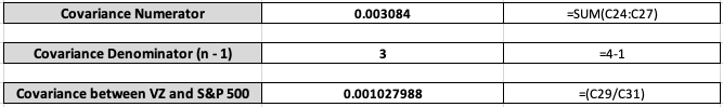
Once this final step is fulfilled, the covariance between monthly returns for VZ and the S&P 500 can be found.
The above calculation shows that the covariance in Verizon and S&P 500 monthly returns stands at around 0.001. This suggests minimal covariance as the resulting output is close to 0.
How to use the COVAR Function in Excel?
Using COVAR in Excel is a more straightforward process; continuing with the previous dataset, one can directly deduce the covariance between Verizon and S&P 500 monthly returns by entering the COVAR function.
This can be done by typing the syntax in a new cell:
=COVAR(Array 1, Array 2)
The method to navigate for COVAR is given below:
After entering the function in an empty cell, the VZ monthly return entries in cells C4:C7 must be selected for Array 1, and the S&P 500 monthly return observations from D4:D7 should be highlighted for Array 2. To find the covariance, one has to close the brackets and press enter.
In this case, the resulting syntax would be
=COVAR(C4:C7, D4:D7)
where, C4:C7 looks at VZ monthly returns while D4:D7 pulls up S&P 500 monthly returns.
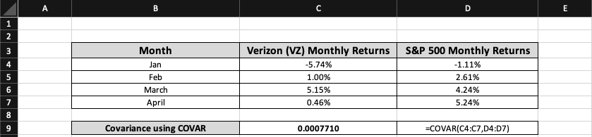
As mentioned earlier, COVAR's output must be converted from percentage to number. When running the COVAR function, the covariance between VZ and S&P 500 monthly returns is approximately 0.0008.
Interestingly, the resulting value produces a different covariance than the manual calculation done in the earlier example. This is because the COVAR function assumes the covariance is of an entire population, whereas the covariance formula focuses on the covariance of a sample.
The subsequent discrepancy can be further explained using Excel's COVARIANCE.S and COVARIANCE.P functions. For instance, if one plugs in the values from the above dataset using COVARIANCE.S, the output would be identical to 0.001 (the covariance formula answer).
However, if COVARIANCE.P is utilized for the same data, the resulting number would be 0.0008 (COVAR function answer).
Interpretation of Covariance Results
Once a covariance value is found, one has to analyze the significance of that number.
It can be broken down into three categories: positive, negative, and zero covariance.
- Positive Covariance: When two variables in a dataset share a positive covariance, it denotes that both will simultaneously experience a general increase or decrease. For example, two securities will record similar price movements if their covariance is greater than zero.
- Negative Covariance: This suggests that the two variables are inversely related. If the covariance is found to be less than zero, it results in variable A facing a decline on the same day variable B sees an uptick. The variables are said to share an inverse association.
- Zero covariance: The linear relationship between two random variables is absent in this rare instance. If the covariance is exactly zero, there is no linear relationship between the two variables, meaning changes in one variable are not associated with changes in the other variable.
Note
If one had to classify where the previous covariance calculations would fall amongst these three categories, the ideal placement would be within the zero and positive range.
The manual formula provided an answer of 0.001, while the COVAR function calculation computed a value of 0.0008. Both figures are close to zero covariance, but the minuscule positive numbers suggest that they cannot share the characteristics assigned to absolute zero covariance.
Hence, there is a very slight chance that VZ and S&P 500 monthly returns will move upwards or downwards together.

Free Resources
To continue learning and advancing your career, check out these additional helpful WSO resources:


or Want to Sign up with your social account?