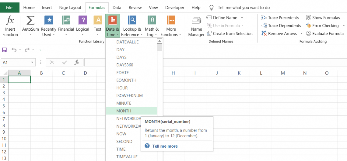
MONTH Function
One of the Date & Time Functions in Excel that returns the month part as a number from a given date.


What is the MONTH Function?
The MONTH function is one of the Date & Time Functions in Excel that returns the month partly as a number from a given date. Depending on the data supplied to the function, the value returned can range from 1 to 12, corresponding to January to December.
Excel stores data in serial numbers from 1st January 1900, corresponding to serial number 1. Thus, 2nd January 1900 would correspond to serial number 2.
Even though the dates are stored as serial numbers, Excel allows us to extract the day, month, and year components of the dates using the functions present in the library.
As a financial analyst, extracting the month from a date has many practical applications, such as grouping the bonds that pay off coupon payments in the same month, preparing rent rolls, etc.
This article will help you understand how to use the MONTH function and the scenarios in which you will likely use it.
Key Takeaways
- The MONTH function is an Excel Date & Time Function that is used to extract the month component from a date.
- Users provide a date as the argument to the MONTH function. It returns the month component of the provided date as a number between 1 (January) and 12 (December).
- The function is commonly used in data analysis tasks, such as trend analysis, seasonal analysis, and historical data comparison, by extracting the month-from-date values for further analysis.
- Potential errors that users might encounter when using the MONTH function, such as providing non-date values or referencing cells with incorrect data, and how to address them effectively.
How the MONTH function works
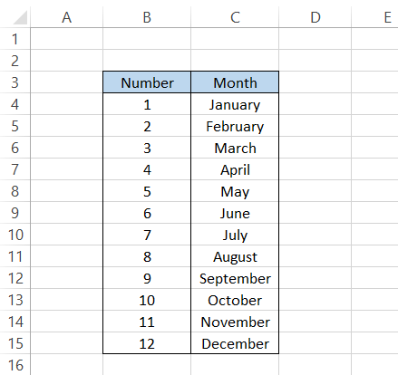
The MONTH is categorized as a Date and Time function that returns a number between 1 to 12, representing the twelve months from January to December in a particular year.
When you reference or hardcode a date in the MONTH function, say 8-May-2022, we will get the result as five or the fifth month, which equals May.
Similarly, if the enclosed date is 12/4/2022 and the function returns the number 12, we have extracted the December month.
The syntax for the function
The syntax for the function is:
=MONTH(serial_number)
where,
- serial_number = (required) a serial number, the cell containing the date or a formula that returns the date which will be used to extract the month
Please note, As you know, dates can also be represented as serial numbers. For example, the dates in Excel begin from 1st January 1900 and hence occupy the serial number position as 1.
Similarly, if you have the date as 4th December 2022, then the corresponding serial number will be 44899.
Examples of MONTH Function
We have illustrated several forms you will often see in Excel to understand how the function works with different date formats.
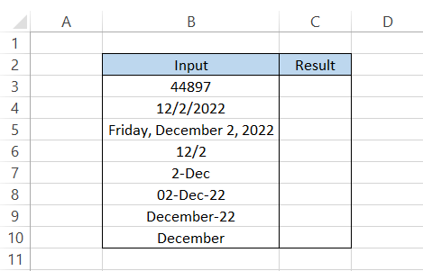
The date is the same, i.e., 2nd December 2022, but it can be represented in several formats from our beloved format cell dialog box.
The formula we will use to extract the month from the date is =MONTH(B3) which will give you the same result in all the cells in column D.
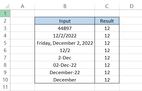
This proves that even if you write the date in any of the readable formats in Excel, the function will efficiently work to return the month component from the date.
WSO Tip
Getting errors for wrong date formats inserted in Excel can be pretty standard. If you are a person who makes a lot of mistakes in date formats, say input date as DD-MM-YYYY instead of MM-DD-YYYY, then we recommend you use the DATE function.
The function takes in three arguments - year, month, and date in the same order. So, if you need to input the date as 14th December 2022, then the formula will be =DATE(2022,12,14) which should give you the expected result.
a. Practical Example #1
Assume that you have a portfolio of several bonds. The bonds pay a semi-annual coupon payment, for which you receive an Excel file for any bonds that pay coupons in the next three months.
To group all the bonds and find the total amount receivable from the coupon payments, we can use the combination of the MONTH and SUMIF functions.
Assume that the dataset looks as illustrated below:
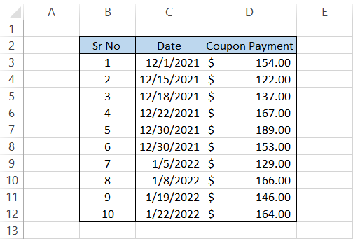
Here, you can directly use the function or the combination of CHOOSE and MONTH functions(explained in the example ahead). We will go with the former option by inserting an additional column for the formula.
The formula will be =MONTH(C3) in column E, which will give you the result:
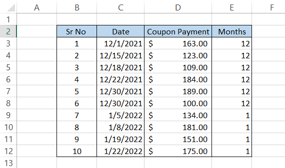
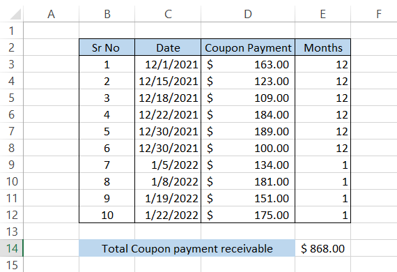
Finally, we will use the SUMIF function such that the formula =SUMIF(E3:E12,12, D3:D12), which will give us the total coupon payments receivable for December as $868.00.
MONTH function vs. EOMONTH function
The most significant difference between both functions lies in their name. A MONTH generally returns the month from the date while the EOMONTH or you can also call it 'End of Month,' returns the last day of the month.
The former function has a primary interest in the month component, while the latter has an interest in the date component.
The syntax for the EOMONTH function is:
=EOMONTH(start_date,months)
where,
- start_date = starting date in Excel from which you need to find the last day
- months = The number of months to go forward or backward in time
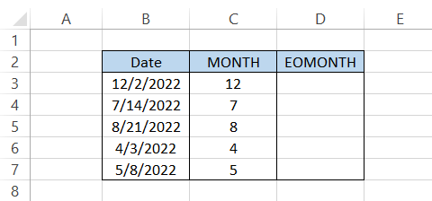
For example, suppose that you have the dates in Excel as illustrated below:
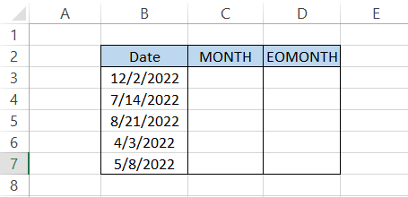
By using the formula =MONTH(B3) in column C, the extracted months for the dates are as illustrated below:
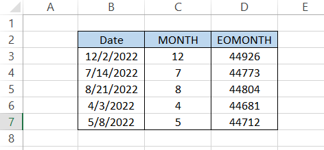
However, on the other hand, by using the formula =EOMONTH(B3,0) in column D, we first get the date serial numbers.
By changing the format to 'Short Date,' the final result would be as illustrated below:
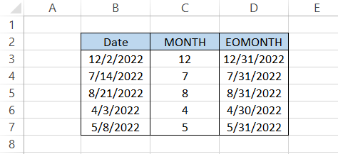
As you can see, the EOMONTH function returns the last date of the month from the start_date, which is different from what the MONTH function does.
It proves that EOMONTH primarily focuses on the day component of the date while the MONTH function focuses on the month component.
Alternative methods to return month
The ability of Excel to perform a similar task but in a different way is quite astonishing. That way, the Excel user can take a different approach in different scenarios.
Suppose you want to extract the month from a date but don't want to break up the data integrity(add or remove additional columns). How would you proceed?
We have listed various alternatives you can use in similar scenarios while working in Excel.
Method #1 - Using the Format Cells dialog box
If you cannot insert additional columns in Excel but need to group the dates into months, we advise using the custom formatting from Format Cells.
- Select the dates from the spreadsheet
- Press the keyboard shortcuts of Ctrl + 1, which should open the window as illustrated below:
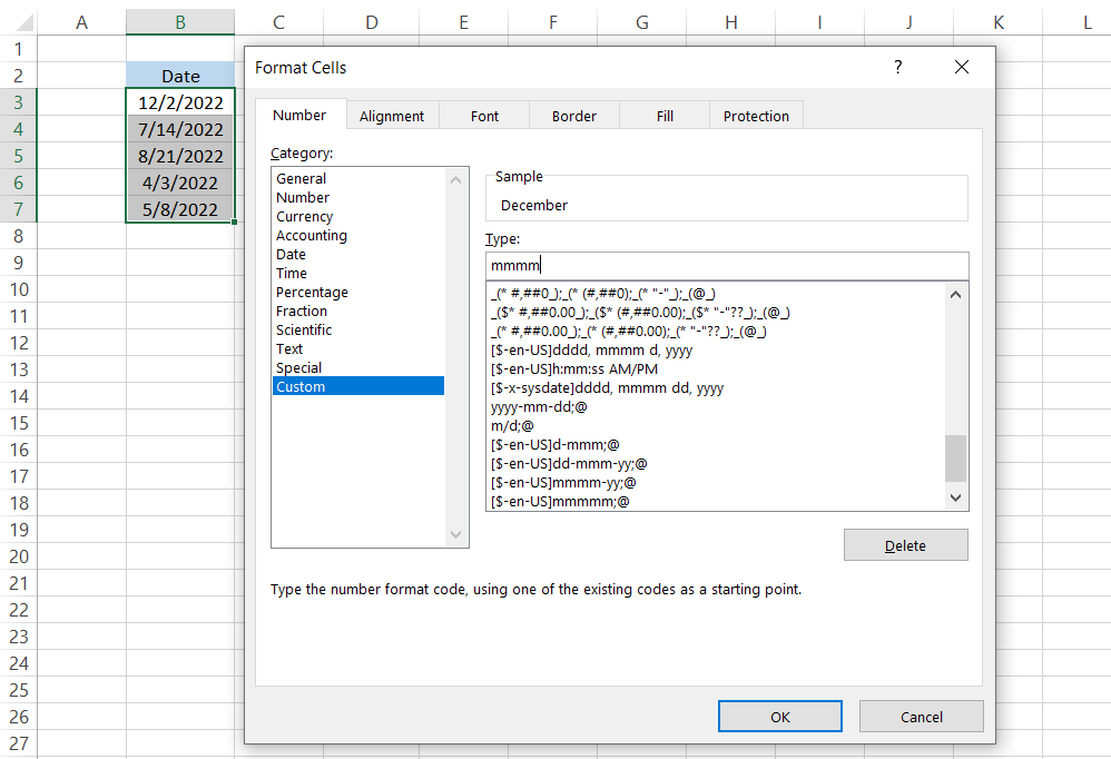
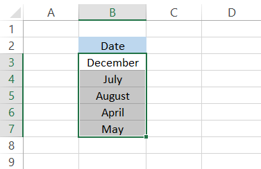
- Click on Custom and type in the custom format as 'mmmm.'
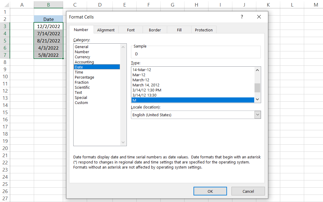
- Once you click on OK, the dates in the spreadsheet should look as illustrated below:
Method #2 - CHOOSE function
The CHOOSE function returns a value from the specified list based on the index number that we input in the formula. For example, assume that you have three fruits on the list:
- Apple
- Mango
- Pineapple
If you input the index number as 2, the return fruit would be mango.
The MONTH function only returns the number corresponding to a particular month. However, using the CHOOSE function, you can directly replace the month's name in Excel.
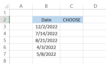
In the example above, if you use the formula:
=CHOOSE(MONTH(B3),"January","February","March","April","May","June","July","August","September","October","November","December")
It will give you the results:
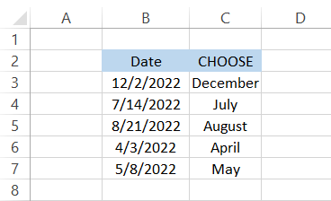
There is just one thing you need to ensure - insert the months in a sequence inside the quotation marks and not randomly, or else the function won't work correctly.
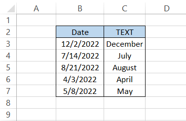
Method #3 - TEXT function
The TEXT function in Excel allows the user to convert numbers into different formats and return the final result as a text string. Since the dates are also numbers, the text function will enable us to extract the months using formatting similar to custom formats.
Remember that we had used 'mmmm' as the custom format to return the months from the dates using the format cell option?
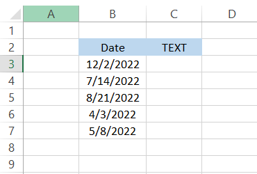
Here, we will use the formula =TEXT(B3, "mmmm") where the format is enclosed within the quotation marks to return the result as:

Free Resources
To continue learning and advancing your career, check out these additional helpful WSO resources:


or Want to Sign up with your social account?