NOT Function
An Excel Logical Function that returns the inverse of the logical statements or the boolean value.


What is the NOT Function?
The NOT function is an Excel Logical Function that returns the inverse of the logical statements or the boolean value.
So, for example, when the conditions are evaluated as TRUE, the use of the NOT function will return the result as FALSE and vice versa.
The NOT is one of the most intriguing functions you might find while working in Excel. Think of the function this way: someone asks you for directions towards Yellowstone National Park, and you tell them, "It’s in the South.”
However, the person surprisingly takes a U-turn and goes all the way toward the North.
Like the example above, the function is added as an intentional element to negate Excel's conditional statement or the boolean value.
We won’t explain why the function is necessary in depth, but for now, let’s remember that everyone has a unique role in this giant universe.
- The NOT function is an Excel Logical Function that reverses the logical value of a statement or expression.
- The NOT function reverses the logical value of a statement or expression. It returns TRUE if the specified condition is FALSE and FALSE if the condition is TRUE.
- The syntax for the NOT function typically includes one argument representing the logical condition to be reversed. It returns the opposite logical value of the specified condition.
- The NOT function performs logical negation, meaning it changes TRUE to FALSE and FALSE to TRUE. It is particularly useful when working with logical expressions or conditional statements.
NOT function Formula
The NOT is a logical function that negates boolean values, i.e., it will return TRUE as FALSE or give the result for FALSE as TRUE.
The function can be used to identify cells that are not empty or that do not meet certain specified conditions.
For example, if you have a list of players who play basketball and football, you can easily identify who doesn’t play football, and the result will be TRUE for all the players who play basketball.
On the other hand, the status for all football players will return as FALSE since we use the NOT function to negate the effect of the logical condition.
Yes, we agree that the function seems confusing on the surface, but it has its benefits in different situations.

where
- logical: (required) a logical statement or a boolean value
That’s another single argument function. Don’t they make life a lot better? Well, we can say that the function might be easier to use than understand. In the subsequent sections, let’s see examples of how the function works.

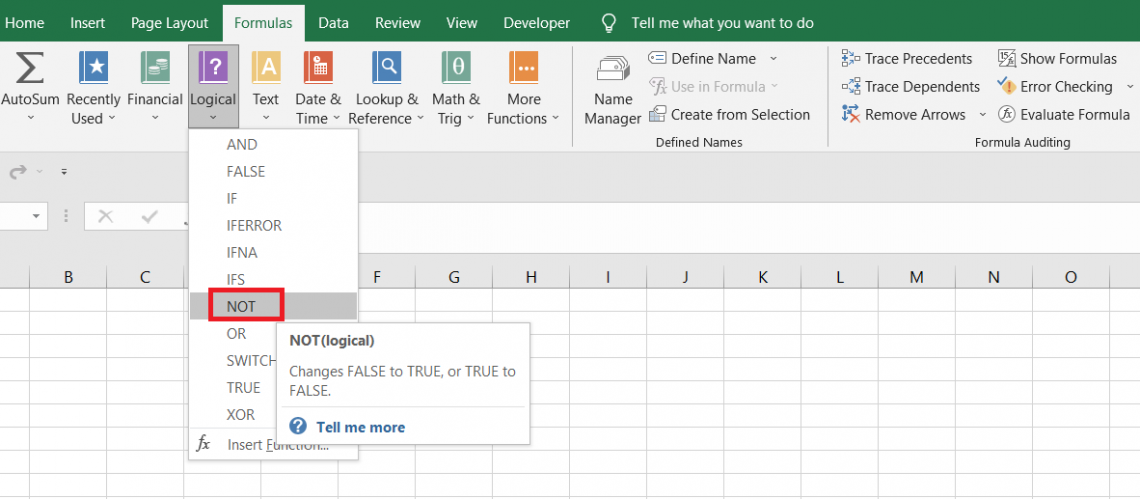
How to use the NOT Function in Excel?
Let’s take a couple of really simple examples to understand how the function works.
Example 1
Suppose you have the Excel data as illustrated below:
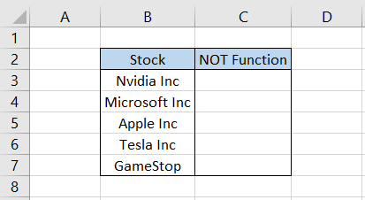
All the stocks were purchased recently in your portfolio. First, you need to determine whether the stock purchased in your portfolio was ‘not’ Nike but any other company stock.
Here, we will use the formula =NOT(B3="Nike") in cell C3 and drag it down till cell C7, which gives the result as
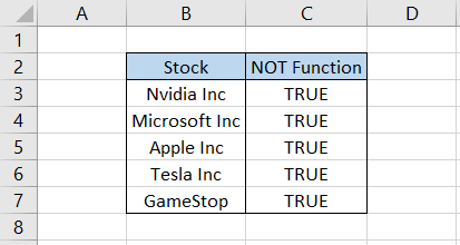
Since all the results are TRUE, Nike doesn’t exist in the portfolio of stocks. On the other hand, if the result evaluates to FALSE, then it means that the particular value is present in the given dataset.
Example 2
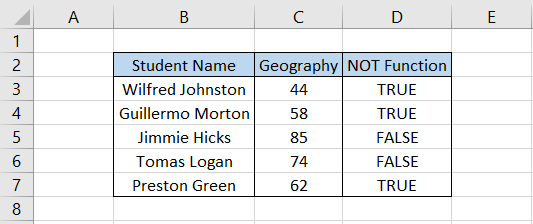
Let’s see how the NOT function and numbers work. Suppose you have the student’s test scores as illustrated below:
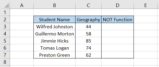
First, we must determine which students have ‘not’ scored test scores above 70.
By using the formula =NOT(C3>70) in cell D3 and dragging it down to cell D7, we get
The COUNTIF function can then determine how often the ‘not’ condition was fulfilled after using the function.
The formula will be =COUNTIF(D3:D7,"FALSE") in cell G4, giving the result as 2.
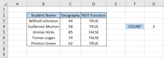
Thus, in two instances, the test scores in Geography were not greater than 70. If we hadn’t used the NOT function, the results would have been inverse; all the TRUE would have been FALSE and vice versa.
NOT Function Practical Examples
Suppose you decide to go on a road trip with a couple of friends and shortlist five cities you can visit. The data looks as illustrated below:
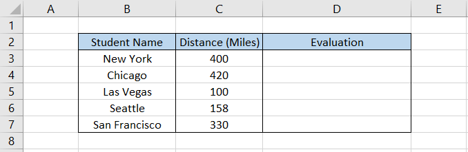
You decide that whatever cities fall within 250 miles of your current position will be one of the first destinations on the road trip.
As you might have already guessed, we will use the IF function such that the formula becomes =IF(C3<250,"Current Destination","Skip for now"), which gives the result.
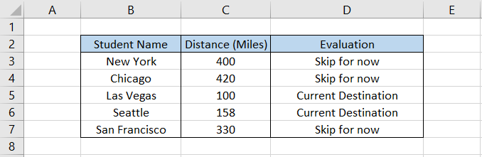
Out of five cities, two could be the potential destination for the first stop of the road trip. Let’s say you decide to travel to cities farther away than 250 miles. Now, you don’t need to change the condition in the formula.
All you need to do is add the NOT function such that the formula becomes =IF(NOT(C3<250),"Current Destination","Skip for now") to give the result
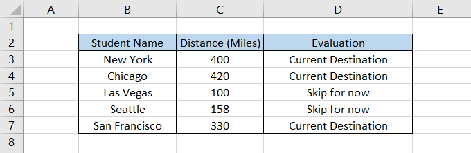
As you can see, the results have flipped without even changing the condition. If there were two different conditions, one evaluates to TRUE and the other to FALSE; then both logical values would also flip like their results.

Free Resources
To continue learning and advancing your career, check out these additional helpful WSO resources:


or Want to Sign up with your social account?