T.TEST Function
A statistical function in Excel that calculates the probability related to a student's t-test.


What is the T.TEST Function?
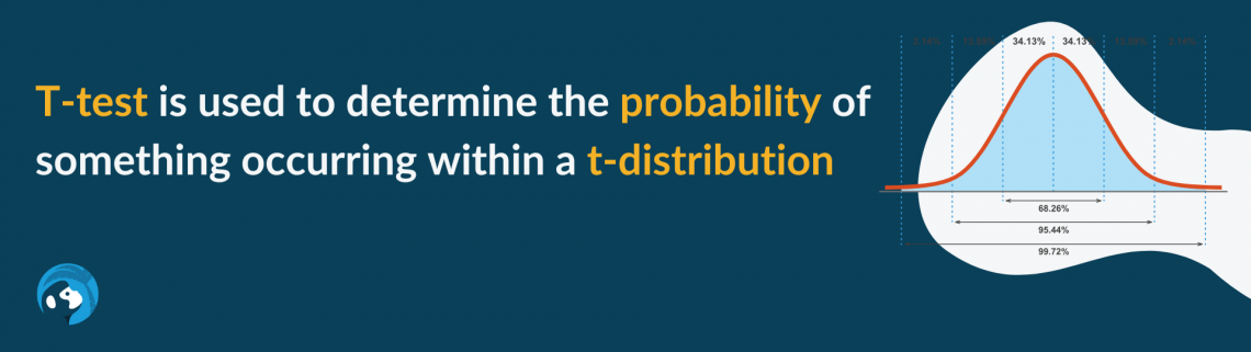
T.TEST Function is a statistical function in Excel which calculates the probability related to a student's t-test. The results of the T.TEST function are used to compare the means of two different samples and ascertain if the difference is statistically significant.
Excel has various functions to aid users in calculating a t-test and determining the probability of something occurring within a t-distribution.
William Sealy Gosset discovered the t-distribution when working for a beer company and trying to find the most optimal ingredients for the beverage. He published the study under the pen name “Student,” which is why it is often referred to as the “Student t-distribution.”
While Gosset used the distribution to determine the crops to use in a beverage, this distribution has implications across many disciplines, as t-tests are a helpful tool to assess differences between populations.
For example, a school may want to determine if there is a significant difference in test scores for students who take a class virtually vs. those taking the same class in person. Tests like these help a school determine whether or not it should administer more online classes.
Calculating a t-test by hand can get complex, so using an Excel function could make it easier. The most commonly used t-test function in Excel is T.TEST. However, this article will discuss other functions and their uses.
- The T.TEST function is used to perform a Student's t-test, a statistical test that determines whether there is a significant difference between the means of two independent sample groups.
- Users provide arguments to the T.TEST function, including the ranges of the two sample groups and, optionally, the tails (indicating a one-tailed or two-tailed test) and the type of t-test (paired or two-sample equal variance or two-sample unequal variance).
- The T.TEST function aids researchers and analysts in deciding the significance of observed differences between sample groups in research studies, experiments, and quality control processes.
- The function is = T.TEST(array1,array2,tails,type). Where array1 and array2 are the ranges that encapsulate each array. Tails are either 1 to indicate a one-tailed test or 2 to indicate a two-tailed test.
The statistics behind the t-test
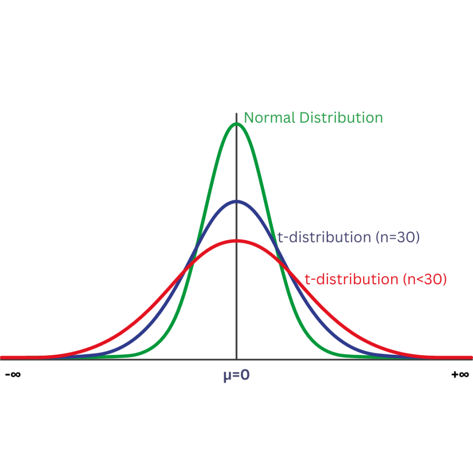
A t-distribution is not the same as a normal distribution. As can be seen in the graph below, a normal distribution has more data clustered around the mean (μ), while the t-distribution is slightly more spread out.
There are three types of t-tests:
- 1 sample t-test
- 2 sample t-test
- Paired t-test
These tests are similar theoretically, with differences occurring when carrying out calculations. We can discuss the steps of any t-test before diving into each specifically.
Step 1: The first thing to start with is creating a null hypothesis (Ho) and an alternative hypothesis.
The Ho in all three tests indicates that the compared values are the same, whereas the H rejects this and indicates the values are different and there is a difference between them.
Then, an alpha (α) value must be determined. This is the significance level; if our final value is greater than the α value, there is a high probability we got the results we did by chance.
Note
When doing a problem in a statistics class, the problem will usually indicate the α value, but if not (and in real-world applications), 5%, or .05, is commonly used.
Step 2: Calculate the test statistic. This is the part that is quite different for each of the tests.
Step 3: Calculate the degrees of freedom.
It is calculated by subtracting one from the sample size. The degrees of freedom are important as each t-distribution graph based on it is slightly different.
The degrees of freedom and α value are used when referencing the t-value chart to determine the t-value. For example, the diagram is shown below:
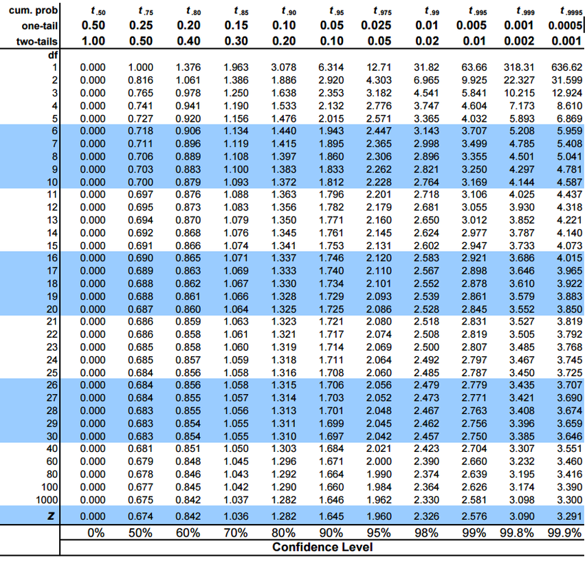
The t-value is compared with the test statistic; if the t-value is greater, there is no statistically significant evidence to prove the null hypothesis is correct, so it is rejected. In its place, the alternative view is found to be true.
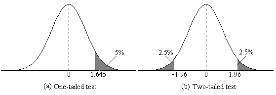
Something to point out is that you may be looking for a one-tailed or two-tailed test. This means either finding the t-value that is the α value distance away from one of the ends of the distribution or finding the t-value that is half of the α value on either side of the distribution.
This can be seen more clearly in the graph below, where the α value is .05. In a one-tailed test, the singular tail is 5% of the distribution, whereas, in a two-tailed test, each tail is 2.5% of the distribution, which adds up to 5%.
Now that we know the general structure of a t-test, we can explore the specificities of each type.

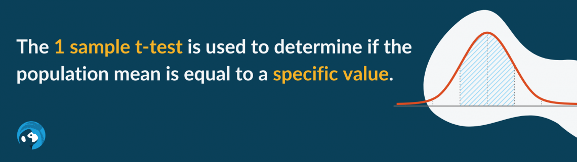
1 sample t-test
The 1-sample t-test determines if the population mean equals a specific value. An example will be determining if the population’s mean heart rate is 110 beats per minute after a 30-minute walk.
The first step is to create Ho and Ha.
H0 : µ = 110
Ha: µ ≠ 110
Next, an α value of 5%, or .05, is assumed as it is not a given.
The next step is determining the test statistic, calculated using the following formula:
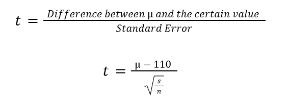
Where
- s is the sample standard deviation
- n is the sample size
The degrees of freedom can be calculated using the following:
df = n - 1
Once this is calculated, the degrees of freedom and α value can be looked up on the t-table mentioned earlier and compared with the test statistic. The final step is to accept or reject the null hypothesis.
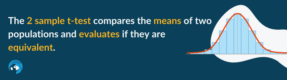
2 sample t-test
The 2 sample t-test compares the means of two populations and evaluates if they are equivalent. An example would be comparing the mean heart rate of men and women after a 30-minute walk.
This test will have a slightly different set of null and alternative hypotheses as this test compares two populations. This can be seen below:
H0 : µmale = µfemale
Ha: µmale ≠ µfemale
Again, the α value will be assumed at .05 because it was not explicitly stated to be different.
Calculating the test statistic is also less similar, as the equation divides the difference in averages over the standard error of the difference.
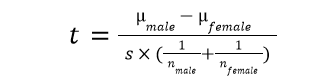
Where s can be calculated using the following formula:
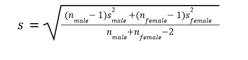
Where
- n is the sample size for each sample
- s is the sample standard deviation for each sample
Once this is done, the degrees of freedom can be calculated using the following formula:
df = nmale + nfemale - 2
Using the degrees of freedom and α value, the t-table can be used to determine the t-value. This can be compared to the test statistic and lead to either the acceptance or rejection of the null hypothesis.
Paired t-test
The paired t-test compares the means of two populations and assesses if the difference between them is 0. This is often used when comparing the variable group to the constant group.
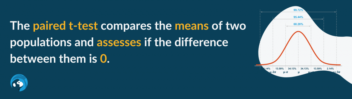
A paired t-test could be used when determining the efficacy of a new drug; if there is no difference in the patient’s well-being, the drug is ineffective.
This is different from a two-sample t-test because the paired test compares samples of the same population when something is done to one of the samples. In contrast, the two-sample test compares samples of different populations.
When conducting a paired test, the corresponding values of each sample are subtracted to get a new data set called the difference.
The beginning steps are the same, i.e., create the hypotheses and determine the α value. Hypotheses for t-tests compare μ to each other or a value, but in a paired test. It compares the difference (hence the subscript d) in population means to 0.
H0 : µd = 0
Ha: µd ≠ 0
Where
µd = µ2 - µ1
The α value is acknowledged to be .05.
The test statistic can be calculated using the following formula:
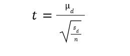
Where
- sd is the standard deviation of the difference data
- n is the sample size of the different data
- μd is the mean of the difference in data
The degrees of freedom can be calculated by doing the following calculation:
df = n - 1
Then, the degrees of freedom and α value is used on the t-table to find the corresponding t-value.
This t-value is then compared to the test statistic; if it is greater than the t-value is greater than the test statistic, it indicates the findings are most likely not found by chance and that there is statistically significant data to reject the Ho.

T.TEST Function Formula
As the lengthy sections above show, calculating a t-test by hand is not very convenient. Excel, however, has created several functions to help users easily calculate these tests.
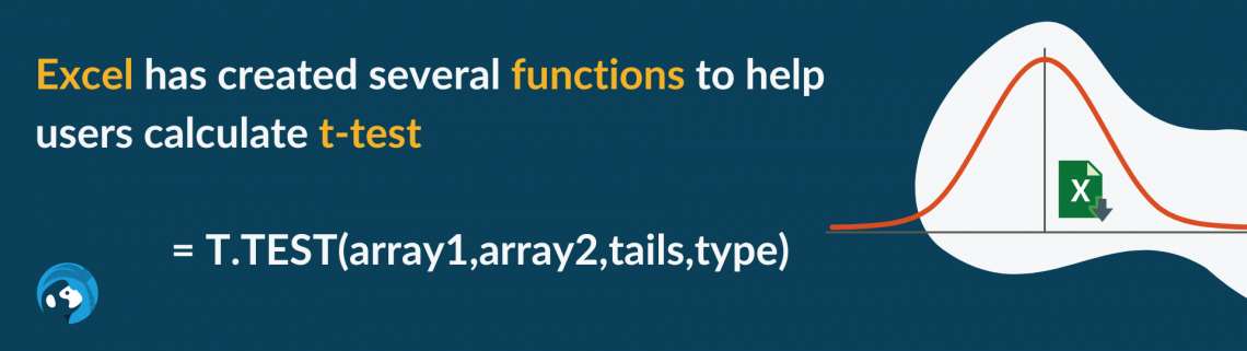
The formula is as seen below:
= T.TEST(array1,array2,tails,type)
Where
- array1 and array2 (both required) are the data sets to be evaluated
- tails (required) defines if the distribution is one-tailed (enter 1) or two-tailed (enter 2)
- type (required) specifies what t-test to perform
- 1 indicates a paired test
- 2 indicates a 2-sample t-test with equal variances
- 3 indicates a 2-sample t-test with unequal variances
The second and third options for type describe how the data is spread apart from a potential regression line (“line of best fit”). If it is consistent throughout the data, two should be used. However, if it changes, three should be used.
How to Use the T.TEST Function in Excel?
Now, we can explore examples using T.TEST. First, we can look at a paired t-test. Say we are trying to determine if the male adult population has the same mean heart rate when resting and after walking for 30 minutes.
Our hypotheses will be:
Ho: μrest - μactive = 0
Ha: μrest - μactive ≠ 0
We will assume an α value of .05.
The formula to solve this would have the following components:
- array1 would contain the data points of the resting heart rates
- array2 would contain the data points of heart rates after walking for 30 minutes
- Tails would be 2, as using a 2-tailed test would check for differences above and below the distributions, not just one side.
- The type would be 1 to indicate we are using a paired test.
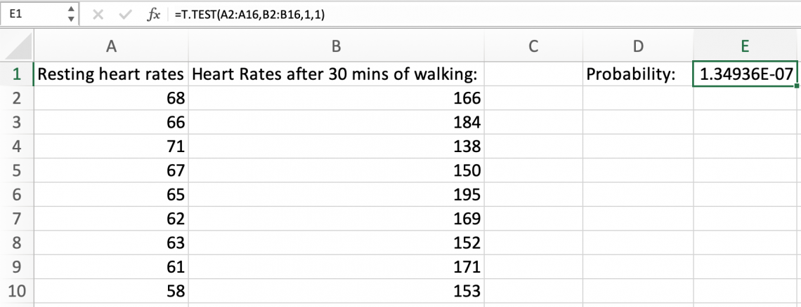
This is the resulting value, and because it is smaller than the α value of .05, we can reject the null hypothesis and conclude that the difference in the means is not 0.
But what if we were comparing samples from two different populations? We would have to use either the second or third options for type.
Say we are trying to determine if there is a difference between male resting heart rates and female resting heart rates. We would have to determine if the variance was the same (or very similar) for each population.
We can assume that the variances are the same for male and female resting heart rates and use a nearly identical formula here as we did for our paired t-test.
Before beginning, we must create hypotheses and acknowledge that the α value is .05.
Ho: μmale = μfemale
Ha: μmale ≠ μfemale
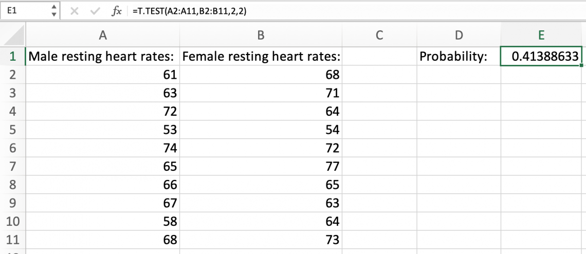
This formula uses the ranges of male resting heart rates and female resting heart rates in a two-tailed test where the variances are the same.
This results in a much higher probability than .05, implying we accept the null hypothesis that the population means the heart rates of males and females are the same.
This is not the case, as females tend to have a slightly higher heart rate than males. However, because our sample size was so small, it is hard to discern such a small difference.
Note
T.TEST cannot be used to calculate a one-sample t-test, as the function requires two array inputs
Additional t.test functions in Excel
There are quite a few functions made for getting more information about a t-distribution on Excel. So, we will look through them briefly and discuss their uses.
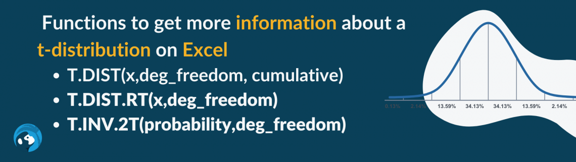
- T.DIST(x,deg_freedom, cumulative): This function is used to find either a cumulative probability leading up to a certain x value or a certain x value occurring in a t-distribution. This is helpful when looking specifically for a left-tailed possibility.
- T.DIST.2T(x,deg_freedom): This function is very similar to T.DIST. However, this is a two-tailed function, meaning it will find probabilities from either side.
- T.DIST.RT(x,deg_freedom): This function is nearly identical to T.DIST.2T. However, this function calculates the right-tailed probability rather than the two-tailed.
- T.INV(probability,deg_freedom): This function is the inverse of T.DIST. It requires the probability of an area occurring, which is the output of T.DIST. The output of this function is the x value that bounds the left tail to get the inputted probability.
- T.INV.2T(probability,deg_freedom): This function is the inverse of T.DIST.T2, as it requires an input of the two-tailed probability of occurring and outputs the x value that bounds either tail.
Free Resources
To continue learning and advancing your career, check out these additional helpful WSO resources:


or Want to Sign up with your social account?