Excel Round Down

What is the Excel ROUNDDOWN Function?

As the name suggests, the ROUNDDOWN function in Excel rounds down a number by reducing the digits after the decimal point toward zero.

There would have been numerous occasions where you performed simple arithmetic calculations, for example, 'a' divided by 'b,' and the result was a decimal number.

A decimal number can generally be of three types:

• Terminating decimals - A decimal number with a finite number of digits after the decimal point. For example, when you divide one by 2, you will get the result of 0.5.
• Recurring decimals - A recurring decimal is a number where the digits keep repeating in the same pattern after the decimal point infinitely. For example, 0.232323232323232, 0.481481481481481481481 etc
• Irrational decimals - Another decimal number where the digits after the decimal point keep repeating infinitely. The major difference that this type of numbers show is that the digits after the decimal are non-recurring. For example, 3.1415926535897932, 0.1526548975315 etc

When we get the arithmetic calculation result in recurring or irrational decimals, linking those values to the rest of the financial model can become challenging. For example, if the risk free-rate in your assumptions spreadsheet is an irrational decimal, it would damage your entire economic model.

How would it damage? All the calculations that you make further would have never-ending digits after the decimal point.

To avoid this, you can use this function, where you reference the never-ending numbers and limit them to the 'n' number of digits after the decimal.

In this article, you will understand the syntax for the function, how to use the function and some examples.

ROUNDDOWN Syntax

It is categorized as a Math & Trigonometric function that reduces the decimal numbers from right by rounding them towards zero.

Suppose that you have a number as 48.497951354. The number has nine digits after the decimal point. However, we do not need those many digits in the number.

Here, the function can help us to limit the digits after the decimal point to two. So the final result we would get using the function would be 48.49.

In school, you would have studied rounding of numbers based on the standard rule that if the digit up to which you want to round lies between 0 to 4, then the value gets rounded down. At the same time, if it lies between 5 to 9, then the value gets rounded up.

For example, if the number is 45.88, the value rounded up to one decimal digit would be 45.9; if the number is 45.23, the result will be just 5.2, rounded down to one decimal digit.

However, the same standard rule does not apply to the function. Irrespective of whether the number lies between 0 to 4 or 5 to 9, when the number gets rounded towards zero when you use the function, i.e., the 'nth' decimal place digit becomes zero.

The syntax for the function

The syntax for the function is:

=ROUNDDOWN(number,num_digits)

number = (required) The number will be rounded to specified decimal places.

num_digits = (required) the number of decimal places that you want to round down the value to

How to use the function

The two ways that you can use the function are either from the function's library or as a worksheet formula.

a. Method #1 - From the functions library

What does a function exactly mean? In simple terms, it is a predefined formula where you just input the arguments in the text boxes and get the result in the selected cell.

To use the function from the library, please follow the steps below:

1. Select the cell in which you intend to get the result.

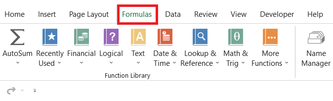
2. Click on the Formulas tab > Math & Trig > select the ROUNDDOWN function from the drop-down menu.

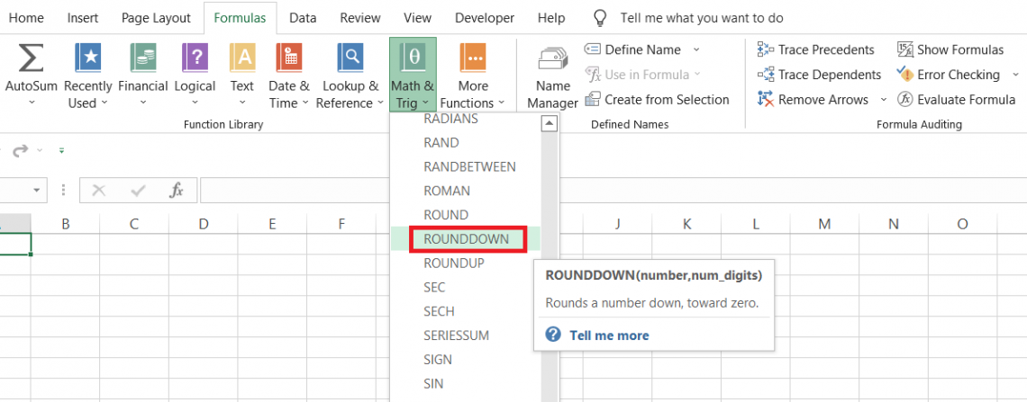
3. This will open up the dialog box as illustrated below:

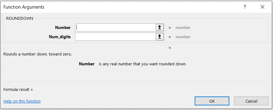
4. Next, we input both arguments. Suppose the number is 3.14159265, and we need to limit the number to only two digits after the decimal. While we know the number argument, the num_digits would equal 2.

You can also reference the cells here instead of hardcoding the values.

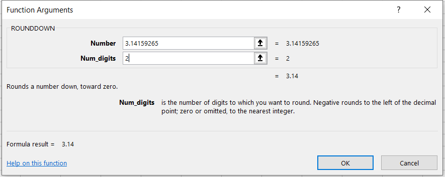
5. We get the preview of our result, which is equal to 3.14. Now, all you need to do is click on Ok, and you will get the same result in the selected cell.

b. Method #2 - As a worksheet formula

If you are looking for the easiest of the two methods, you have come to the correct section of the article. The only prerequisite, however, is that you have good knowledge about different excel functions.

Suppose that we have some numbers in Excel, as illustrated below:

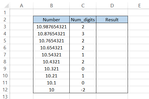
Here, we will use the formula =ROUNDDOWN(B3, C3), which gives the result in column D as:

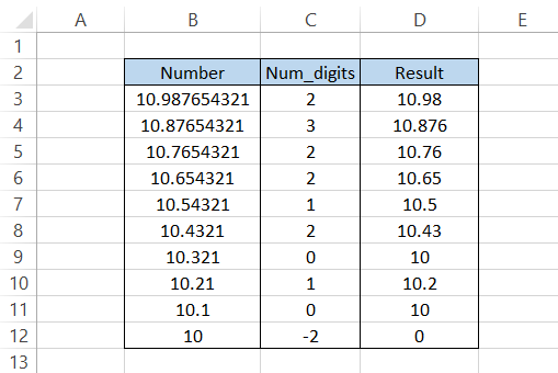
Whatever num_digit we have specified in column C, we get a corresponding result in column D from our given number.

When you input zero as an argument for num_digits, we get an integer value for the number. So, for example, a decimal number 78.95134 will give the result as 78.

If you use a minus one as a num_digit argument, the number in one's place will return as zero. Remember we said that the function rounds down the numbers towards zero? That's what happens.

For example, if the number is 11.1 and you use the num_digits as -1, then the result would equal 10.

A minus two as a num_digit on a two-digit integer would return the number as zero. However, if it's a three-digit number, such as 182, the result would be 100. So the result will only be zero if you use a minus three as a num_digit!

Examples of the function

The function hardly requires in-depth knowledge since it is pretty easy to understand. The function can be used everywhere, from calculating interest rates to maintaining ledger accounts.

The function can be combined with math and trig functions such as SUM, AVERAGE, SQRT, etc.

All you need to do is type in the general formula to get the result. For example, suppose you feel that the number of digits after the decimal is too many. In that case, you nest the result inside this function and limit the digits to your required preference.

For example, if the formula =AVERAGE(A2:A15) gives the result as 8.789465, then by using the updated formula =ROUNDDOWN(AVERAGE(A2:A15),2), you can get the result as 8.78 by limiting the digits after the decimal to 2.

This section will show examples of how the function works with different number formats.

a. Example #1 - Just Números

You already know how the function works if you have numbers in your dataset.

Suppose that you have the interest rates in Excel as illustrated below:

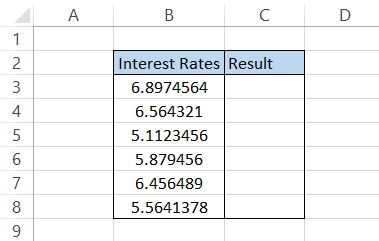
If you want to limit the rates to just two places after the decimal point, you can use the formula =ROUNDDOWN(B3,2), which should give the result:

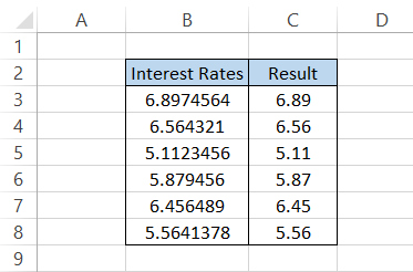
Suppose you have more than two digits after the decimal. In that case, the formula will always return the result with only two numbers after the decimal.

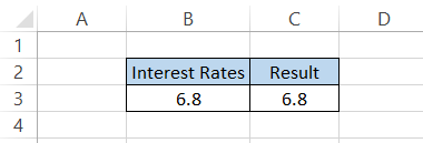
However, the only exception to the formula will be when you have no digits or just one digit after the decimal. In that case, the formula will return the number as it is.

For example, if the number is 6.8 and you use the formula =ROUNDDOWN(B3,2), you would get the same result, i.e., 6.8.

The logic is pretty simple, right?

b. Example #2 - Date and time

Before we understand the effect of this function on date and time, remember this example to alert the readers of a common mistake that can make unintentionally with such data types.

You might never use the function on dates and times, but it's helpful if you know its effect on different data types.

You might know that both date and time are represented as numbers in Excel. To be precise, the dates are represented as integers starting from 1, which is equivalent to the date 1st Jan 1900, while time is represented as decimal numbers.

For instance, if the date is 16th July 2022, the corresponding serial number equals 44758. On the other hand, if the time is 12:00 PM, the corresponding decimal number is equal to 0.5.

Now, you might think the dates don't even have decimal numbers. So the only num_digits that you can input to get a different result is when you use a negative integer.

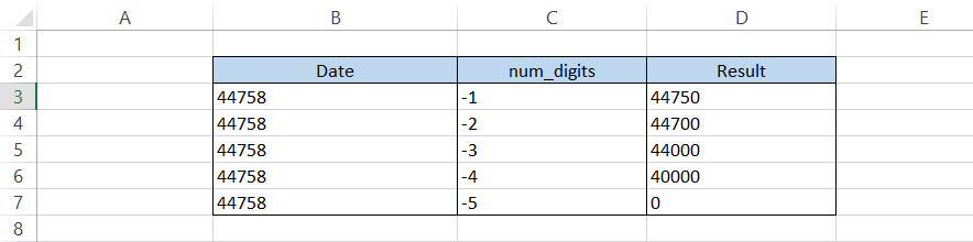
Suppose we have the date in Excel as illustrated below:

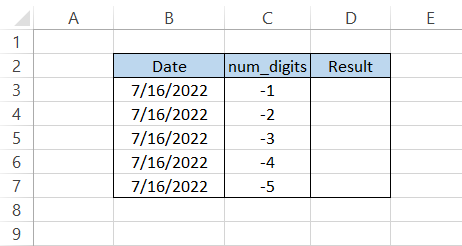
The corresponding serial number for the date is equal to 44758. When you use the formula =ROUNDDOWN(B3, C3) in cell D3 and drag it down to the last cell, we get the result:

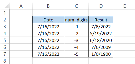
The numbers are turned to zero in positions corresponding to the num_digits argument. For example, if the argument is equal to 4, all the digits up to the thousand's place return zero.

Try copying all the dates in column D and Paste Special using Ctrl + V + V to save the dates as values.

If you press the magic keys Ctrl + ~ on the keyboard, you will see the serial numbers for the date:

Now, the formula's effect might have been effortless to understand!

Similarly, assume you have the time as 9:09 PM in Excel:

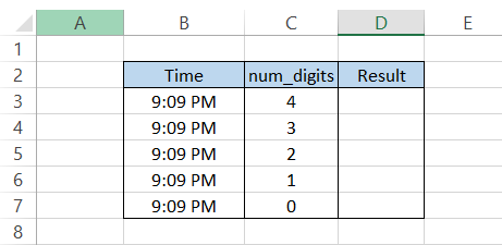
Here, you can primarily use the positive integers to limit the digits after decimal since the time value would be equivalent to decimal values between 0 and 1.

If you use the formula and drag it down up to cell D7, you will get the result:

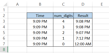
Our time changes as the digits after the decimal turn towards zero. Paste Special those formulae as values in the same column and press the magic keys Ctrl + ~, which would show the corresponding decimal values for the time as:

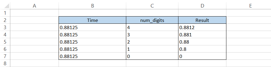
A lot easier to understand what happens behind the scene for date and time when you use those magic keys!

c. Example #3 - Percentages

This is probably the most helpful example of your day-to-day work experiences.

As a financial analyst, you would find percentages in almost all the datasets you work with. Furthermore, these percentage values might have recurring ones, which could be limited to rounded ones.

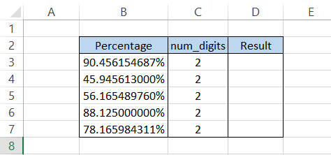
Suppose that the percentage values in Excel are as illustrated below:

By using the formula, we would get the result:

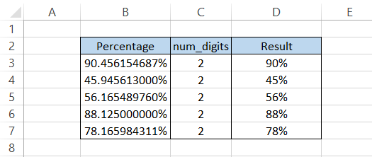
Well, we see a somewhat contradictory result using the formula. Most of us would have thought the result would be, let's say, 90.45% in cell D3.

However, that is not the case.

When you represent a value between 0 to 100 percent, what excel understands is a value between 0 and 1. So if you have the value as 0.35, then it corresponds to 35%.

Suppose it's still confusing to you how things underwent behind the scenes. In that case, we recommend you press the magic keys Ctrl + ~, giving you a different perspective on those numbers.

If you use negative numbers or zero as a num_digits argument, you will get the final result as zero.

ROUNDUP vs. ROUNDDOWN

Let's agree that these functions aren't rocket science. Their names speak up for the 'function' they perform.

A ROUNDUP function, unlike its counterpart, rounds the numerical value away from zero. So, for example, if you have the number 78.9815 and you need to round up the value to three digits after the decimal, then using the function, you will get the result as 78.982.

A phenomenon that you would usually see while using the ROUNDUP function is that whatever digit up to which you round up, that digit value would return away from zero or a plus one. So, for example, 10.231 rounded up to two digits would give 10.24.

The ROUND function rounds up a value only when the digit to the right falls between five to nine, but this is not the case with the ROUNDUP function.

On the contrary, a ROUNDDOWN function rounds the value towards zero.

The syntax for the ROUNDUP function is:

=ROUNDUP(number, num_digits)

where,

number = (required) The number which will be rounded to specified decimal places

num_digits = (required) the number of decimal places that you want to round off the value to

Next, we will see an example of how the result differs for both functions.

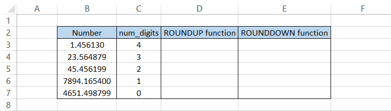
Suppose that you have numbers in Excel as illustrated below:

To find the rounded-up value, we will use the formula =ROUNDUP(B3, C3) to get the result:

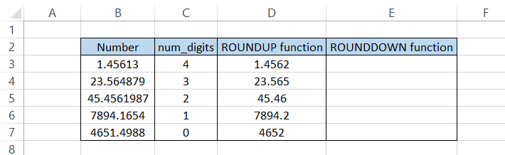
Any digit rounded up till 'n' num_digit is always +1 in our result, i.e., one becomes 2, or 5 becomes six, which is going away from zero. This is the basic principle on which ROUNDUP works.

On the other hand, using the formula, the function returns the number towards zero, i.e., all the numbers at num_digit after decimal become zero.

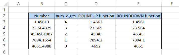
Even though the function performs a similar task, i.e., rounding a value, they return a quite contrasting result.

Researched and Authored by Akash Bagul | Linkedin

Free Resources

To continue learning and advancing your career, check out these additional helpful WSO resources:

• MOD Function
• REPLACE Function
• Types of Graphs
• VBA For Loop
• VLOOKUP