Keynesian Multiplier

What is the Keynesian Multiplier?

The Keynesian multiplier is a ratio that indicates how much output (Y) will change if an exogenous component of aggregate demand (AD) changes by 1 unit.

We can find the Keynesian multiplier model under various names in different economics textbooks. Some economists call it 

• Keynesian multiplier, 
• expenditure or spending multiplier, 
• demand multiplier, 
• simple multiplier, or
• a multiplier or  
• a Keynesian cross.

Samuelson and Nordhouse state in their Economics textbook that the name multiplier comes from the finding "that each dollar change in exogenous expenditures (such as investment) leads to more than a dollar change (or a multiplied change) in GDP."

Also, it is necessary to remember that the fundamental assumptions behind the multiplier model are fixed wages and prices and that the economy is operating below its potential (there are unemployed resources available).

Burda and Wyplosz provide the most general definition of the Keynesian multiplier in their Macroeconomics textbook. A multiplier is "a ratio indicating the effect of increases in exogenous components of aggregate demand on total aggregate demand."

Another definition is provided by Rittenberg & Tregarthen (2009) in their Principles of Economics. The multiplier is "the ratio of the change in the quantity of real GDP demanded at each price level to the initial change in one or more components of aggregate demand that produced it."

"The multiplier is the impact of a 1-dollar change in exogenous expenditures on total output. In the simple C+, I model, the multiplier is the ratio of the change in total output to the change in investment" (Samuelson & Nordhaus, 2010).

The multiplier effect proved helpful when explaining the business cycles, which are the frequent and unpredictable fluctuations in output, prices, and employment. The multiplier explains how the shifts in aggregate demand could produce business cycles. 

Exogenous Components of aggregate demand

There are four exogenous or independent components. The same components are also variables of GDP when calculated using the expenditure approach. They are as follows:

• The households' Consumption of C
• The firm's Investment I
• The Government's Purchases of G
• The foreign markets' Net export Nx

1. Consumption (C)

In most cases, consumption is the GDP's most significant component. It refers to the households' expenditures on goods, mainly food and shelter. The consumption of goods such as clothing, recreation, and automobiles is also significant. 

2. Investment (I)

We must understand that we use the word 'investment' when addressing any process or action of investing money for profit. Mainly, it is used to name investments in financial markets.

Economists agree that the term 'investment' can generate confusion. When talking about the components of aggregate demand, we are, restricting the word 'investment' to the activities that increase the economy's stock of capital (including buildings, equipment, software, etc.). 

3. Government Purchases (G)

Governments purchase goods from firms and households. It is essential to mention that there is a difference between government spending and government purchases(G). Not all government spendings are a component of aggregate demand. 

For example, transfer payments (mostly welfare payments to households) are government spending but not government purchases. The government will not receive any good or service in return for the transfer payment. 

4. Net Export (Nx)

Net Export is calculated as Export less Import:

Net Export (Nx) = Export (X) - Import (I)

Export represents all the domestic goods and services sales abroad, and Import reflects all the foreign goods and services purchases.

The net Export could be in the form of a trade deficit when Export is lower than Import. On the other hand, if Export is higher than Import, the net Export could be a trade surplus. 

Keynesian multiplier economic analysis

The general idea is that the increase in AD is more significant than the initial increase in one of the AD components. 

Multiplier =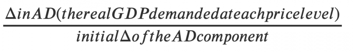  

Caption- Source: Rittenberg & Tregarthen (2009)

The Keynes multiplier doctrine is based on the propensity to consume and save. 

According to Keynes (1936), the economic concept of multiplier was first introduced by R. F. Khan in 1931 in his article 'The Relation of Home Investment to Unemployment.' 

R. F. Kahn, while explaining the multiplier concept, stated that "the change in the amount of employment will be a function of the net change in the amount of investment." 

However, Keynes explains his multiplier in the famous work 'The General Theory of Employment, Interest and Money,' published in 1936.

The multiplier in the simple model C+I is directly related to the marginal prosperity to save (MPS) and marginal prosperity to consume (MPC). Under this model, it is crucial to explain the relationship between savings, consumption, and investment. 

The savings and consumption relationship is described as follows: As savings is that part of disposable income that is not consumed, we can say that:

Savings (S) = Disposable Income (DI) - Consumption (C)

Savings and Investment relationship

Under the national accounting rules, the measured saving is the same as the measured investment. We determined this relationship from the following (assuming there is no government and foreign sector):

Investment (I) = Product - Approach GDP - C

Savings (S) = Earnings - Approach GDP - C

Therefore:

Investment (I) = Savings (S)

Keynes (1936) defined the propensity to consume and to save as "the result for the community as a whole of the individual psychological inclinations how to dispose of given incomes." 

1. The marginal propensity to consume (MPC)

It is the additional amount people consume when they receive an extra dollar of income. We would calculate it as the first derivative of the C (Consumption) function.

MPC = C'

2. The marginal propensity to save (MPS)

It is the additional amount people save when they receive an extra income. We would derive it as the first derivative of the S (Savings) function.

MPS = S'

3. The relationship between MPC and MPS

MPC + MPS = 1

MPS = 1 - MPC

MPS is identical to 1 minus MPC, meaning that each dollar not spent for consumption is spent for savings. 

The multiplier, also called the Keynesian spending multiplier, is as follows:

Multiplier = 1/ 1 - MPC

or

Multiplier = 1/ MPS

The multiplier can also be named according to the aggregate demand or GDP component, impacting the output or GDP. 

For example, suppose the changed component is the investment, and the multiplier is the number by which the change in investment must be multiplied to determine the resulting change in total output.

Then, the impact of the simple investment multiplier on the output (GDP) is as follows:

Δ in  output =

Δ in  output = 

The equations above are adopted from Samuelson and Nordhaus' textbook on Economics (2010). They focused on the simplest multiplier, which is an exogenous variable investment. 

According to this textbook, the Keynesian multiplier model shows that an increase in investment will increase GDP by an amplified or multiplied amount - by an amount greater than itself. 

In his original work from 1936, Keynes focused on the impact of government purchases and tax cuts on the GDP. Therefore, let us define the government expenditure and tax cut multipliers. 

When discussing the government expenditure multiplier's impact on the GDP,  we mean the following:

Δ in  output =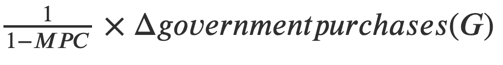  

Δ in  output =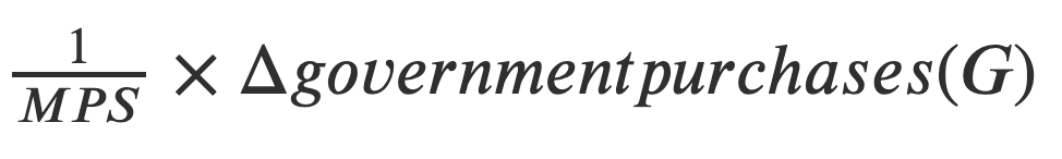  

In the equations above, the 1/MPS and 1/(1-MPC) are the multipliers. As it is clear from the equations above, the higher the MPC, the higher the impact of additional government purchases on the GDP. 

tax cuts and the GDP

According to Charles R. Nelson's Macroeconomics (2006), the tax cut stimulates the economy during a recession. 

Therefore, the tax cut impact also has a multiplication effect. However, the result is indirect, as the tax cut increases household income. Increased disposable income leads to higher consumption. 

Taxes ↓ => Disposable Income (DI) ↑ => ↑ in Consumption (C) by DI X MPC

Also, the savings will increase when the Disposable income is increased. 

Taxes ↓ => Disposable Income (DI) ↑ => ↑ in Savings (S) by DI X MPS

In creating the tax cut multiplier, we need to consider that the tax cut is an actual negative tax change. Therefore, the tax cut multiplier is always minus the government expenditure multiplier less one.

Tax Cut Multiplier = [-1/(1-MPC)] - 1

or

Tax Cut Multiplier = [-MPC/(1-MPC)]

or

Tax Cut Multiplier = -MPC/ MPS

Adopted from Charles R. Nelson's Macroeconomics (2006).

The Keynesian Multiplier model is often used as an argument for supporting fiscal stimulus during an economic recession. It is important to note that the multiplier effect is only valid while unemployment exists in the economy; the economy is operating below its potential.

Also, the New Keynesian economic school, widely accepted today, is not supporting the traditional Keynesian multiplier model. 

Calculating the Keynesian Multiplier

Keyness explained the mathematical background of the multiplier in his work "A Treatise on Probability" (Chapter 26) in 1921. In the footnote of Chapter 26, he reflected on the process of the limit of a declining geometric infinite series for the calculations used to support his theory of risk (page 360). 

The mathematical logic is later applied in Keynes' work from 1936 on explaining the multiplier. However, according to Keynes alone, Khan introduced the multiplier concept in economics in 1931. 

The mathematical analysis of the multiplier logic can be explained with the following example (adapted from Samuelson & Nordhaus, 2010). Suppose a company hires an unemployed resource to build new software. 

The company pays the resource (developer) 1000 dollars. The 1000 dollars is an initial investment change that will impact the output. As we learned from the economic analysis of the multiplier, the difference in production will be more significant than the initial change in investment. 

The question is, how much does the output increase more than the initial investment? To find an answer, we must realize that the initial investment money will continue to flow within the economy.

Our developer will spend a part of the income on goods, resulting in the money flowing to the producers of those goods. How much the developer would spend on the goods is reflected by the marginal propensity to consume. 

If the developer's marginal propensity to consume is ⅔, the developer will use 666,67 dollars to buy consumption goods. The producer of these goods will now have an income of 666,67 dollars. The producer's MPC is also ⅔. Therefore, they will spend 444,44 dollars.

The process can also be reflected and calculated as an infinite geometric progression. A general endless geometric progression is as follows:

1 + r + r² + r³+ r⁴+ r⁵+ ... + rⁿ + ... = 1/(1-r)

In the equation above, r is MPC. The formula is valid if the r (MPC) is less than 1 in absolute value. We can apply this formula to the case of MPC as follows:

1 + MPC + MPC²+ MPC³+ ... + MPCⁿ = 1/(1-MPC)

This is how we derive our multiplier in mathematical terms. We can use this knowledge in our example and calculate the impact of the increased investment of 1000 when the MPC is ⅔ of the output (real GDP). 

1/ (1-2/3) x 1000, or 3 x 1000 = 3000

It is clear from the mathematical analysis of the multiplier that the higher the MPC, the higher the impact of additional investment on the GDP. For example, if MPC is 0.5, the multiplier is 2. If the MPC is 0.9, the multiplier is 10. 

We can repeat this example by considering other components of Aggregate demand (or GDP), such as government spending or consumption. Some sources call the multiplier also the government expenditure multiplier (considering the impacts of government purchases). 

Keynesian multiplier Graphical explanation

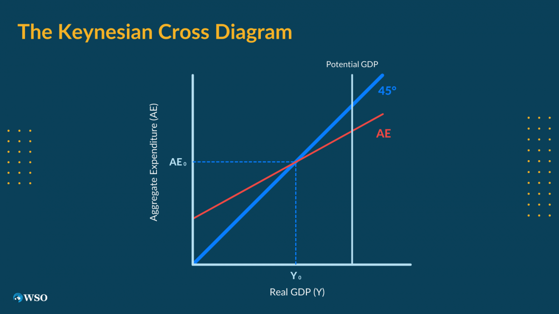
The Keynesian multiplier model is often graphically represented on the Keynesian cross diagram. The name cross comes from the way the model looks. The aggregate demand (or aggregate expenditure) curve or line crosses the 45° curve. 

The graphical diagram of the model is also called

• the expenditure-output diagram
• the Keynesian cross diagram
• the 45° diagram

The expenditure-output (Keynesian cross) diagram reflects the equilibrium level of real GDP at the point where it is equal to the aggregate (or desired) demand. It also reflects that the economy is operating below its potential GDP (output) level. 

In other words, the 45° diagram shows how output adjusts to desired demand under the Keynesian assumption of sticky prices. 

The axes of the diagram are the total output (or real GDP) on the x (horizontal) axis and aggregate demand (aggregate expenditure or desired demand) on the y (vertical) axis.

The multiplicator effect is evident when we demonstrate a change in any of the independent components of aggregate demand on aggregate demand on the graph. Let us consider an initial increase in government purchases  ΔG.

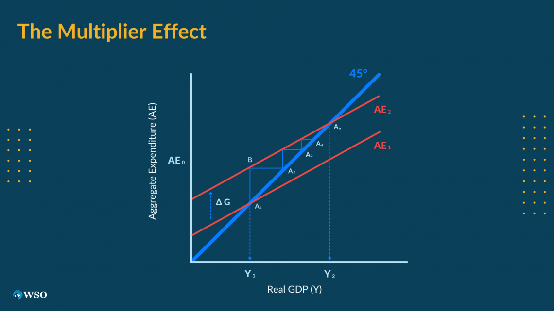
After the change in government purchases, the AE will move from AE1 to AE2. The increase in Y, from Y1 to Y2, is much higher than the increase in G. To explain this situation, we use the multiplicator effect.

The initial increase in expenditure will impulse further economic spending, increasing aggregate demand or expenditures (AE). The effect is illustrated as moving up a staircase from A1 to An.

Researched & Authored by Katarina Gajdosova | LinkedIn

Reviewed and edited by Parul Gupta | LinkedIn

Free Resources

To continue learning and advancing your career, check out these additional helpful WSO resources:

• Demand Theory
• National Currency
• Public Goods
• Seller's Market
• Exchange Rate