Marginal Rate of Substitution (MRS)
The rate at which a consumer would be willing to give up one good in exchange for another while remaining at the same level of utility


What Is The Marginal Rate Of Substitution (MRS)?
In microeconomics, the marginal rate of substitution (MRS) is the rate at which a consumer would be willing to give up one good in exchange for another while remaining at the same level of utility. It is a key tool in modern consumer theory and is used to analyze consumer preferences.
As previously noted, the marginal rate of substitution is a consumer’s willingness to forgo a good in exchange for units of another good while remaining at the same level of utility. In other words, MRS puts the marginal utility of one good in terms of the other.
Marginal rates of substitution are calculated between commodity bundles of goods x and y on a common indifference curve. Because indifference curves are usually curved, the slope of the line changes as you move along the curve.
Various combinations of goods x and y that result in equal utility for the consumer are plotted on the indifference curve.
The slope of the curve at each bundle reveals the exact combination of goods that brings a consumer equal satisfaction as any other bundle on the curve. So, in essence, the marginal rate of substitution is the slope of the indifference curve at a single point.
When modeling consumer preferences for normal goods, MRS is diminishing. I.e. As one consumes more of good x, one consumes less of good y because they are substitutable to a certain degree (shown by the MRS).
- MRS measures the rate at which a consumer is willing to exchange one good for another while maintaining the same level of utility. It quantifies consumer preferences and is used in modern consumer theory.
- MRS is calculated as the ratio of the marginal utilities of two goods, representing the slope of an indifference curve. It signifies the trade-off between goods while keeping satisfaction constant.
- Indifference curves plot combinations of goods that yield equal utility. The slope of the curve at each point indicates the MRS, revealing the goods’ substitutability or complementarity.
- For normal goods, MRS is diminishing. As consumption of one good increases, consumption of the other decreases due to their substitutability to a certain extent.
- MRS analysis doesn’t account for bundles preferred over the current one or for comparing different bundles. It is generally limited to analyzing two-variable situations or functions. There can be misconceptions about MRS treating goods equally; it actually considers the change in the quantity of goods for equal utility.
How to Calculate Marginal Rate of Substitution?
The marginal rate of substitution between two bundles on an indifference curve is easily represented as y/x, which is the rate of change formula. This is the easiest method to use when solving for MRS.
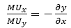
The formula for the Marginal Rate of Substitution is:
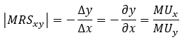
where:
-
x, y = two different goods
-
dy/dx = derivative of y with respect to x
-
MU = marginal utility
The rate of change formula is the easiest method to use when solving for MRS and is easiest when using two points on a graph. However, indifference curves are not typically straight lines, so finding the marginal rate of substitution at a single point can be tricky without a graph.
There are two ways to calculate MRS at a single point. The first is by way of brute force: calculating the slope of a line that lies tangent to the indifference curve. This method, however, tends to give rough approximations. The more common method is to use calculus.
Using calculus to find the marginal rate of substitution is the most common method when using a function.
Graph and Function Examples of Marginal Rate of Substitution
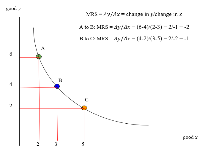
The graph below depicts three commodity bundles on the same indifference curve. Using our formula, we find that our theoretical consumer gives up 2 units of y to acquire 1 unit of x when moving from bundle A to bundle B. Thus, the MRS when moving from A to B is -2.
Similarly, we also find that the consumer gives up 2 units of y to acquire 2 units of x when moving from bundle B to bundle C, yielding an MRS of -1.
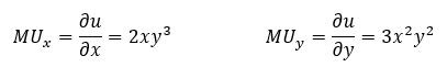
Finding the MRS at a specific point on the indifference curve is easy when using a utility function.

Now that we have a function, we take the partial derivative of U with respect to x and y.
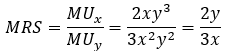
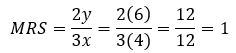
Then, plug these inputs into the MRS formula and simplify.
The final step is to plug your point into the formula. For the purposes of this example, we’ll use (4,6).
Limitations of the Marginal Rate of Substitution
The major drawback in evaluating the marginal rate of substitution on a single indifference curve is that there is no mechanism to account for a commodity bundle that a consumer prefers over his existing bundle.
One would have to examine multiple indifference curves to identify bundles that would yield greater utility. Even in this case, the mathematics involved do not distinguish between bundles on different curves.
Furthermore, MRS analysis does not examine commodity bundles composed of different goods that a consumer might prefer to his current bundle. Only those bundles composed of the same goods can be examined.
As such, MRS analysis is typically limited to two variables, unless given a function with three or more variables. Such functions would yield a graph with three or more axes, which is difficult to imagine.
Even in this case, the analysis only examines bundles composed of different quantities of the same goods.
Watch the following video to see an example of calculating MRS using a function with three variables.
Misconceptions of Marginal Rate Of Substitution
A commonly held misconception of MRS analysis is that it presents the utility of two substitute goods equally, despite that a consumer may prefer to have a bundle composed of all of one good. This assumption is not entirely true.
Let’s examine two bundles on the same utility curve. Because they lie on the same curve, they must yield the same utility.
Thus,
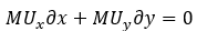
Based on the example above, we know that marginal utility of one good is the change in utility that results from altering the quantity of that good in a bundle.
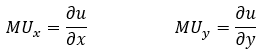
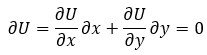
So, a bundle’s change in utility is the result of the change in quantity of goods x and y. Taking the partial derivatives of U(x,y) with respect to x and y, we get:
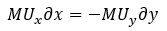
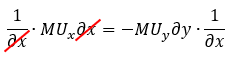
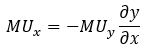
Subtracting the second term from both sides of the equation, we are left with the following:
From this example, we can see that the utility of two goods in a bundle is not treated equally. Rather, it is the change in the quantity of x and y when moving between bundles that are considered to have equal utility.
Thus, there is an inverse relationship between the two goods, such that increased consumption of one offsets the decreased consumption of the other to keep utility constant.
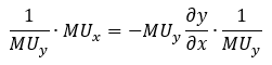
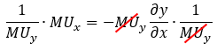
Deriving the MRS Equation
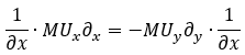
By further manipulating the equation above, we can derive our original formula.
So, after all that math, two things become clear:
-
MRS analysis does not treat the marginal utility of goods in a bundle equally. There is an inverse relationship between the two goods, such that increased consumption of one offsets the decreased consumption of the other to keep utility constant.
-
The marginal rate of substitution is equal to the ratio of the marginal utilities, which is equal to the slope of the curve at a commodity bundle.
We can take this one step further. A key assumption in economics is that consumers always seek to maximize their utility relative to what they can afford. To examine exactly how a consumer does this, we use a budget line.
A budget line, or budget constraint, represents all possible combinations of x and y that a consumer can afford to buy, given the price of the goods and the consumer’s income.
Individuals prefer to consume where the budget line is tangent to the indifference curve because that is the bundle that maximizes the consumer’s utility relative to what he or she can afford.
Thus, we know that the slope of the indifference curve at a utility-maximizing bundle is equal to the slope of the budget line. This can be represented by the following:
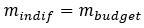
Furthermore, because we know that MRS is equal to the ratio of the marginal utilities, MRS is also equal to the ratio of the prices.
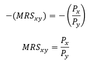
At this utility-maximizing bundle, MRS = Px/Py because consuming below the budget constraint would mean being on a lower indifference curve, yielding less utility. This equality is important because it tells us that the marginal utility of per unit of money spent is equal for each good.
MRS and Indifference Curve
Indifference curves connect commodity bundles composed of two goods. Each bundle on the curve represents a unique combination of the two goods. Consumers are “indifferent” when choosing between bundles on the same curve because they yield the same level of utility.
A graph that depicts multiple indifference curves is called an indifference map. Think of it as a topographical map, where contour lines represent different elevations. Similarly, on an indifference map, each curve is associated with a different level of utility.
Like topographical maps are two-dimensional representations of a three-dimensional landscape, an indifference map is just a two-dimensional representation of a three-dimensional utility surface, which is just a visualization of a utility function.
As we have already demonstrated, MRS is the slope of the indifference curve at a specific bundle. The most common indifference curves model normal goods that are moderately substitutable, like hamburgers and pizza.
These curves are convex towards the origin because as an individual consumes more of one good, he consumes less of the other. As such, the marginal rate of substitution diminishes as one moves to the right.
However, indifference curves come in a variety of shapes. For example, if the goods in question are inferior, then individuals prefer to consume less of each good. In this case, indifference curves would be concave towards the origin and MRS increases.
Indifference curves that model two inferior goods are considered to be non-monotonic and non-convex.
Other commonly seen shapes exist when modeling goods that are infinitely substitutable or non-substitutable at all.
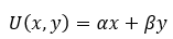
When modeling perfect substitutes, like a dollar bill versus another dollar bill, indifference curves do not take on the typical convex shape. Instead, they look like diagonal lines that connect the x and y axes.
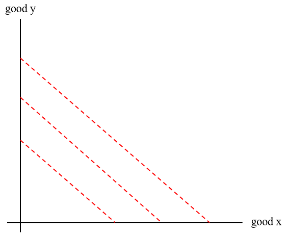
Since the two goods are perfectly substitutable, the exchange rate between them is fixed. As such, the MRS remains constant along indifference curves for perfect substitutes.
In general, utility functions for perfect substitutes take on the following form:
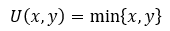
Whereas perfect substitutes are infinitely substitutable, perfect complements cannot be substituted at all.
Consider left shoes and right shoes. They are sold together because, given their perfect symbiotic relationship, there is no benefit to giving up one for the other. As such, there is no exchange rate at which one could trade left shoes for right shoes.
Perfect complements are modeled by the following:
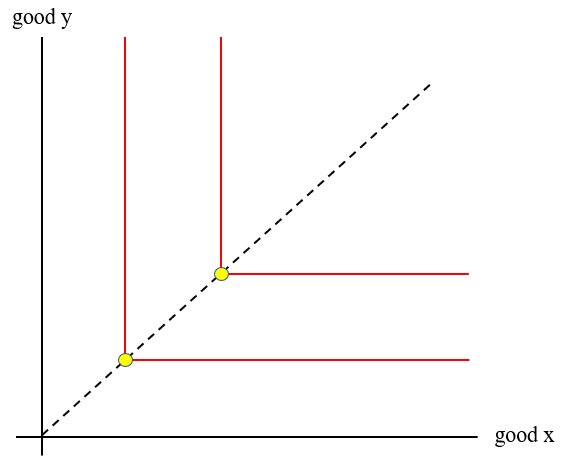
The MRS for perfect complements is infinite along the vertical portion of the curve, 0 along the horizontal portion of the curve, and undefined at the corner.
And because perfect complements are worthless without each other, utility comes from whichever good in the bundle the consumer has less of:
To find out how MRS and indifference curves fit into the broader study of economics, check out our article on microeconomics.
Economists understand market dynamics and how macro events affect them, which tends to make them good investors. If you have a background in economics and are interested in a career in finance, check out our modeling, interview, and exam prep courses here.
Marginal Rate Of Substitution (MRS) FAQs
MRS stands for the marginal rate of substitution. It is the rate at which a consumer would be willing to give up one good for units of another without sacrificing satisfaction.
The concept of diminishing MRS holds true when modeling normal goods. I.e. goods that have rising demand during periods of rising income.
If MRS > Px/Py, the consumer will consume more x and less y. If MRS < Px/Py, the consumer will consume less x and more y. If MRS = Px/Py, the consumer will not change their consumption because MRS = Px/Py where the budget line is tangent to the indifference curve.
Marginal utility is the additional utility someone receives from making a certain decision. For example, let’s say someone’s total utility is 10. That person then decides to buy an ice cream cone. After eating it, his total utility is 12. The marginal utility of buying the ice cream is 2.


or Want to Sign up with your social account?