Microeconomics
The science of individual behavior and choices under restrictions, known as scarcity


What Is Microeconomics?
Microeconomics is the science of individual behavior and choices under restrictions, known as scarcity. Since we live in a world with limited resources, we must allocate them efficiently to maximize optimization and benefits effectively.
Microeconomics has two main agents involved in this dimension, consumers, and firms. The decision-making problems are the core of microeconomics.
The interaction between supply and demand creates a new field, the Price Theory. This interaction will be different in each scenario, with a few producers or demands, only one, etc.
Thus, microeconomics is a powerful tool. You can apply it in many fields, including policymaking and even macroeconomics. The modern macroeconomic models have micro-foundations.
One of the main characters of this "revolution" was Robert Lucas. and his Critique of the Keynesian macroeconomics models.
To him, there was no sense in trying to forecast a policy's effect only with historical data. Policymakers must have their models based on rational decision-making instead.
F.A. Hayek had some credits on it too, but this time in a philosophical aspect. His paper "Scientism and the Study of Society" has some insights on it. Analyzing the macro phenomenons without understanding agents' actions does not hold rational value.
Remember, this article is an overview of microeconomics to motivate you to study more. Other articles in WSO give a deeper view of each topic; look at them; their link will be throughout the article.
Method of Microeconomics
A very relevant discussion before entering microeconomics is to understand its methodological problems. It is crucial to prevent elementary mistakes, such as confusing "rationality" in economic theory and common sense.
There are three main microeconomics methodology discussions:
1. Normative vs. Positive Economics
The definition of Positive Economics is often viewed as more analytical, and it says "what is." While Normative is more idealistic and says "what should be."
To Milton Friedman, all economics, while science, must be positive. The normative can be the one that says "what should be" but must show the reason for things to be in the way it's saying.
If you say that the world should be less unequal, you must give a reason, how to do it, and the method's effectiveness. Thus, all economics, in a scientific way, is positive. Every policy must have empirical foundations and pass rigorous studies.
2. Methodological individualism
A characteristic of social sciences is that they work with organizations acting like individuals. In economics, we deal with a firm like it was an individual, with motivations, etc.
Every institution's aggregate behavior is the output of the behavior of its parts. So, to understand the macro phenomena, we must understand how its functions behave.
An increase in interest declines consumption. You can see it by plotting a graphic and seeing the correlation.
The graphic can tell you if there is a correlation, but not the reason for this phenomenon. How the agents will behave under more extensive interests is what matters. Only this allows us to comprehend the macro effect.
Macro phenomena are the output of aggregated micro-agent behavior.
3. Models and their unrealistic assumptions
The critics of the unrealism of economic models don't make any sense. All models are the simplification of reality, even in physics. A model is created precisely to do this, to isolate a phenomenon and study it.
The only way to not have any simplification is to look at the entire system.
The argument "models are useless because the economy is complex" it's the exact reason to use them. The analysis of the entire economic system cannot happen at once.
Another misinterpretation is seeing a model as an empirical fact. Instead, models are simplifications that explain specific cases but won't work for them all.
Milton Friedman explains in his essay 'The Methodology of Positive Economics. In his words:
"Only factual evidence can show whether it is "right" or "wrong" or, better, tentatively "accepted" as valid or "rejected." [...], the only relevant test of the validity of a hypothesis is a comparison of its predictions with experience."
There are some critics of Friedman's theory. His error was that the assumptions don't need to be false. Thus details aren't missing, and they are negligible.
Another critique is that the model doesn't have value for its predictive power. In his paper "Credible worlds: the status of theoretical models in economics," Sugden says that a model's value is its explanatory power.
Consumer Theory
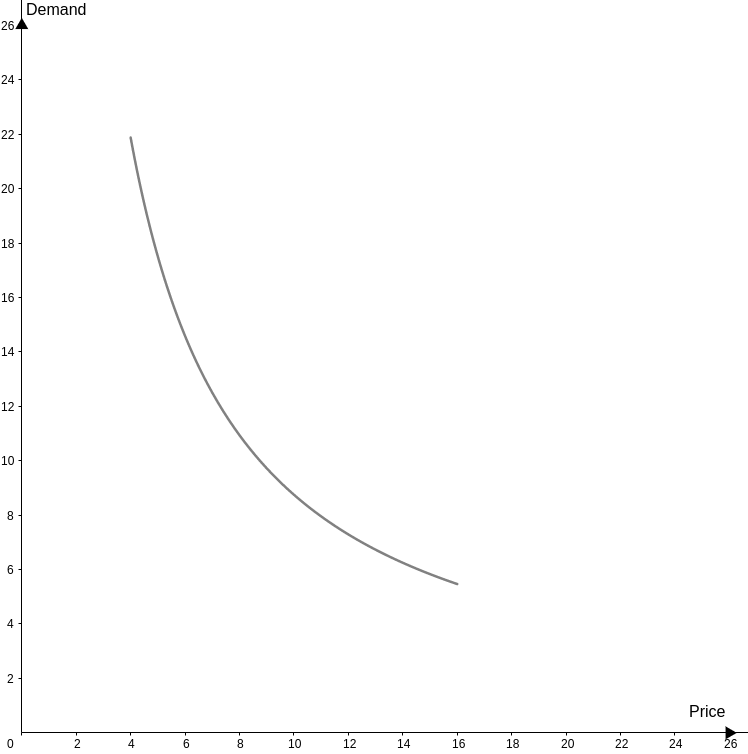
In microeconomics, it's important to understand how the demand curve forms.
The demand is just a consequence of agents' behavior in front of their incomes and the good's prices. This is what we'll learn here, how people behave and allocate resources under budget constraints.
The consumer theory has its assumptions:
-
Perfect information; A consumer is aware of the commodities used for consumption, and all knowledge is given to them about a product using excellent information where there are no gaps for missing information or critical product details.
-
Agents are price takers; consumers cannot change the market price and must pay the price determined by the market.
-
Prices are linear; if prices are linear, there's no quantity discount. Thus, consumers with more purchasing power will not have marginal benefits
-
Goods are divisible. Products can be divided into smaller units for consumption and retain the same linear value. Rational behavior is a central theme to understand in Microeconomics. It is important to comprehend preferences and their implications to understand what rationality means.
Preferences
Consumers' preferences are built axiomatically. An axiom is a self-evident proposition. From the axioms, we can derive relations and construct the theory on them.
The consumer's behavior axioms are
-
If a and b are both goods. If a is better than b, then b ≺ a.
Read as "a is strictly preferred to b."
-
If a is at least as good as b, then a ≽ b.
Read as "a is weakly preferred to b."
-
If b is as good as a, then b ∼ a.
Read as "a is indifferent to b."
Now you already know how to read the notation so that I can introduce the axioms of consumers' behavior:
-
Completeness: the consumer has complete preferences if, and only if, given two good x and y, then, x ≽ y or y ≽ x.
-
Transitivity: the consumer has transitive preferences if, and only if, given three good x, y, and z, then, if x ≽ y and y ≽ z, thus x ≽ z.
You won't work with only one good. The problem is about the choice between two or more things. Thus, we deal with a set of goods, and it is denoted in brackets. Let's see an example with two goods to make it easier.
Imagine a consumer that has apples and pears, and he is willing to exchange two apples for one pear. This implies that if he must choose between one apple or one pear, he'd choose the pear, thus apple ≺ pear.
The Law of Diminishing Marginal Utility implies that for each new pear, the consumer will lose satisfaction with the product over several uses and purchases; thus, there will be a certain number of pears that will make him prefer an apple; in contrast, according to the Law of Diminishing Marginal Utility.
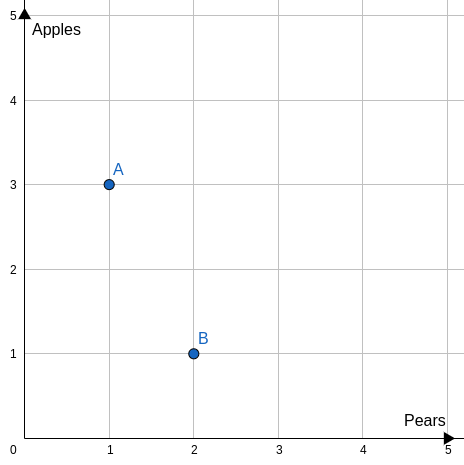
Both sets {3,1} and {1,2} give the same utility to the consumer, that is {3,1} ∼ {1,2}, next you’ll learn what is an indifference curve, everything will be more clear.
In microeconomics, we assume that the consumer is insatiable. That is, more is better. Thus, {x,y} ≺ {x,y}, for any greater than 1:
To make things easier, we must have something to calculate the “satisfaction” of this consumer. But how do we do it? Here is where Utility Functions appear.
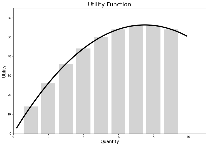
Utility functions
Economists optimize Utility Functions to model the preferences mathematically.
The utility functions translate consumers' behavior into a mathematical equation.
A utility function U quantifies consumer satisfaction for buying something. It can have only one input or as many as we want. We can translate the preferences to utility functions notation:
-
b ∼ a if, and only if, U(a) = U(b)
-
b ≺ a if, and only if, U(a) > U(b)
-
a ≽ b if, and only if, U(a) ≥ U(b)
The most used utility function is the Cobb-Douglas type. It has its advantages because it is convex in all its domains. The definition of a Cobb-Douglas utility function is
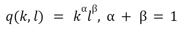
When we add more goods to our function, we do not have a 2-Dimension graphic, and you'll have a 3-DImension graphic. As it is hard to work with 3D graphics, economists use the indifference curves:
-
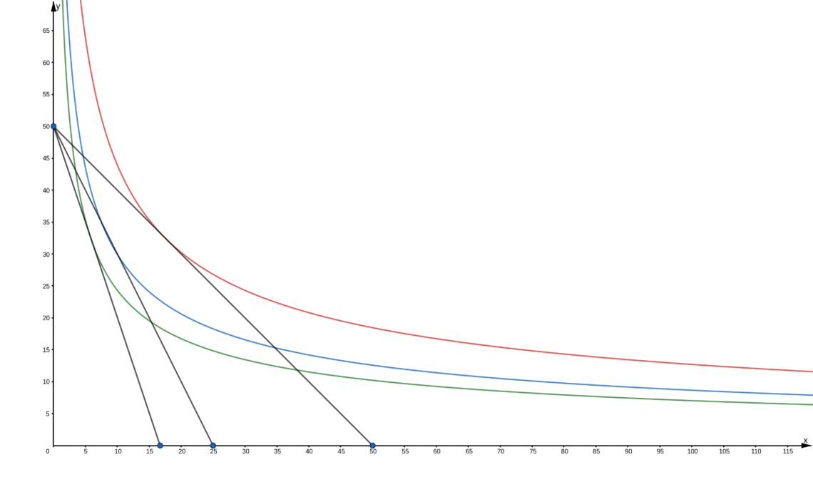
Indifference curves are the level curves of the utility function. They represent all the combinations between both goods that give the same utility.
The indifference curves are the abstraction of the preferences relation. If someone is willing to exchange two units of something to have more of another in both combinations, he'll have the same satisfaction. The indifference curves display it.
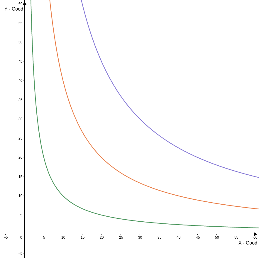
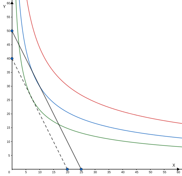
The graphic shows the indifference curves of a Cobb-Douglas utility function where both goods have the same weight. The red line is to u(x,y) = 30, the blue line to u(x,y) = 20, and the green to u( x,y) = 10.
Marginal Utility and MRS
Marginal analysis is one of the main tools for economists. In Consumer Theory, frequently, we want to have the Marginal Utility of one good in the set. This is when we use mathematics; to be more specific, we use derivatives (calculus).
In a utility function with only one good, it's easy to derive the process. A derivative is the variation tax of a function at a specific point. To do it is to make the ratio between the function variation when the quantity of good variation is tiny.
Things get a bit worse when we add more goods to the function. But to simplify, you need to assume that the other good is constant and only variate the one you're working with.
Example: be u(x,y). To find the marginal utility of x, we assume that y is constant; the notation will be:
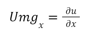
The symbol means "partial." You do not need to know the mathematical foundations or how to prove them. Remember that the marginal utility of x is how much the utility function will variate if only x variates.
With the marginal utility, we can introduce the Marginal Rate of Substitution and its formulas. The MRS measures how much a consumer would give up to have more from others and have the same "satisfaction."
The easier way to calculate the MRS is by choosing two points in the indifference curve and dividing the goods' variations. Using the same consumer from the beginning as an example, what is his MRS? (Remember that Δ means variation)
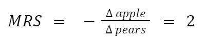
The MRS of apples to pears is 2; he is willing to exchange two apples for one pear. This method is easy, but there is another one that uses marginal utility. The mathematical formula is the following.
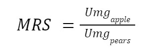
We won't show the mathematical proof here, but if you had a multivariable calculus course, it'd be easy.
Constraint
Limited resources pose constraints.
There are a few vital underlying assumptions:
1. There's no access to credit.
2. The consumer doesn't save anything.
The first assumption is important because we're working with a fixed period. So adding credit to this equation forces us to deal with time in our model.
The second is to make clear that the consumer spent everything he gains. Imagine that investing, in this case, is the same as buying the right to receive the invested capital + interests in a period.
Let's continue. Using the same utility function from the previous section, suppose that the y good cost $2 and x costs $4 to the consumer, so his restriction is given by:
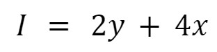
It's equal because we've assumed that the consumer doesn't save anything.
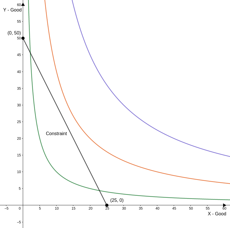
To plot it, we need to imagine what would happen if he spent all his income on only one good?
With it, we'll find where the constraint intercepts the axis, i.e., how much of one good he can buy by giving up all of the other, and in our example, it is
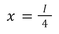
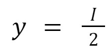
If his income equals $100, he can buy 50 units of y and 25 of x. In the graph, the coordinates of these points will be (0,50) and (25,0). Our constraint line is the segment that links both coordinates:
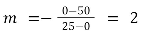
An important thing to know is to find the inclination of the constraint.
Remember that the inclination of a line (m) is given by two dots and the ratio variation of the y-axis between the points and the variation on the x-axis:
Giving a general formula:
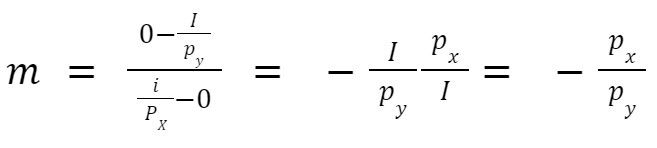
In our case:
Utility Maximization
Determining the most effective method of allocating income is known as the 'Consumer Problem.'
To measure how much would a maximizer consumer spend on each good, economists use the Lagrangian Multipliers.
Using a Cobb-Douglas utility function as an example, Py is the price of good y, and Px x's good. The quantities that maximize the utility is.
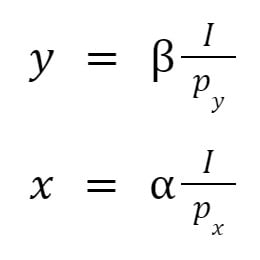
As we have diminishing marginal utility, there is a quantity of good y where if we add one more, we'll have less extra utility than adding one unity of x.
As you can imagine, if we have a function with more than one good, the output will be the same. If you spend all your income on a set of goods, the quantity of each is its "weight" in your utility function, times how much you could buy from it.
Knowing it, we can start to ask some questions. If the price changes, what will happen? And the income? Here we add more dynamics to our model, but this will take a new section about how these changes affect the demand.
Changes in Price and Income
Looking at the demanded quantity, it is easy to see what will happen if the income increases, the demand increases too, and as the price increases, the demand decreases (actually, some goods do not follow this rule; they are known as Giffen’s Goods).
As the individual demand for a specific good is:
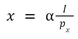
See how the individual demand curve is formed in the indifference map.
If the price increases, the intercept in the axis will change; consequently, the optimum set of goods will also change.
U(x,y) = (x^0.35)(y^0.65)
The price of y will always be $5, and only the x price will change. Our consumer has an income of $250. Let’s see what happens with his indifference map when the x price changes:
The demanded quantity of x changes too. This variation can be sawed in this graphic:
For the demand curve to dislocate, the income must change. This is known as the Income Effect.
Income Effect (xI) is how much demand for goods varies given a variation in the consumer’s income. The Income effect tells us if the good in question is inferior or normal:
-
The consumption of Inferior goods declines as the income increases.
-
The normal goods are the ones that the consumption increases with the income.
Working with the actual examples, suppose that the prices of x and y are constants now. The y price is $5, and the x price is $10. What happens if the consumer income falls from $250 to $200?
The dashed line in the new constraint. If we add price changes, in this case, we’ll see what happens with the individual demand curve.
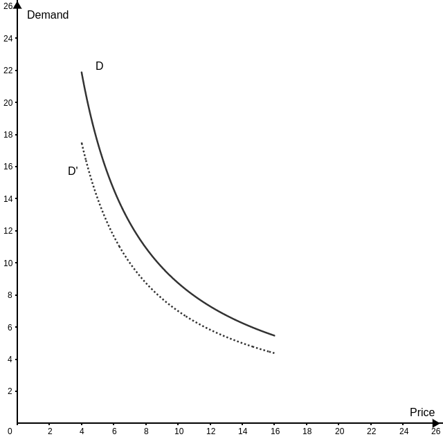
The new demand curve (D’) shows that when the income changes, the entire demand curve dislocates.
Production and Supply Theory
The market equilibrium depends on the supply curve. So, what motivates the firms to produce will create a strong understanding of the supply curve. Without a doubt, profit is what motivates the firm. But, how can profit be maximum?
We'll deal with this now, how much a firm will sell and the distribution of inputs that cost less to make this quantity as profitable as possible.
Let's start:
-
Production Functions: a firm can have many inputs, but to make things easier, we generalize everything as capital (K) or labor (L). The output is the produced quantity with these two inputs combined in different proportions.
-
Cobb-Douglas has many different production functions, but the most used is the Cobb-Douglas. The function is
-
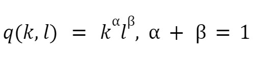
-
Isoquants: Working in 3D graphics is complicated, and we use level curves. It's the same as indifference curves; every curve in the indifference map has all the combinations between capital and labor that give the same quantity.
-
Marginal Rate of Technical Substitution (RTS): the RTS is the slope of an isoquant. This means that this measures how much of k we can exchange for l, and the output will be the same. We have two different ways to calculate it:

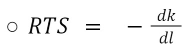
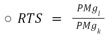
-
Returns to Scale: the returns to scale were first observed by Adam Smith when he looked at the pin factory.
Keeping the capital constant and increasing the number of employees, the factory increased production many times the production inputs.
This case is an increasing return to scale, i.e., the production increases faster than the inputs. There are two others:
-
Constant: the variation of the production is always proportional to the variation in the inputs.
-
Decreasing: the production variates less than the inputs.
Production Costs
One of the main differences between Economics and accounting is how both sciences work with costs. Economists are much more concerned about the company's future, while accountants work mainly looking at the company's past.
There are many different treatments. Some things that accountants would ignore are essential to economic analysis and vice versa. The economic cost is everything under enterprise control and everything, i.e., related to the production process.
We have four different kinds of costs in Microeconomics Theory:
-
Opportunity Cost: economics is haunted by scarcity, we are always trying to find the most profitable business, but our resources are limited. Would you operate a firm that makes less revenue than others?
-
Sunk cost: something that already happened, and there's no way back. Nothing can compensate for this kind of cost. Therefore, it is irrelevant to the decision-making process.
-
Fixed costs: predictable and constant. The only way to be free of them is by stopping the company's operation.
-
Variable costs: costs related to the production process, thus, are proportional to the production volume.
-
The average cost is the total cost divided by the quantity.
-
Marginal costs: how much do costs vary divided by the variation of quantity. If we work with a small variation will find the derivative from the costs function.
To make it easier, we work with the following formula:
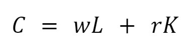
Where r is the cost of capital and w is the labor cost. This equation generalizes the expenses of production. Now we already know each kind of cost, and we'll see it in graphical analysis.
Let's simulate the operational costs of a company and create a spreadsheet:
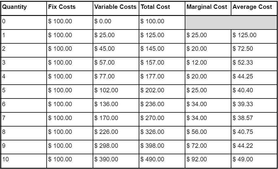
See that the marginal cost declines, reaching its minimum at $ 12.00, and then starts to increase. If we look to a more general marginal cost curve, in the short run, it will always have a u-shape:
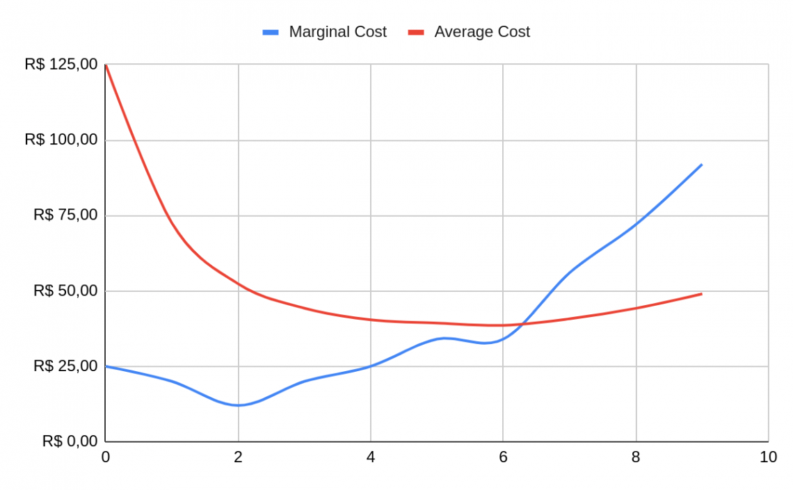
While the average cost starts having a vast decline, this is because of the increase in the produced quantity, and then starts to grow slowly.
The explanation is that the marginal product is smaller than the marginal cost. That is, the quantity produced for each new unity of input increases less than the cost.
It’s important to know that the marginal cost curve differs in the long and short run. In the long run, the firm had much more capacity to change the quantity of the inputs, which doesn’t happen in the short run. Most times is e.

Costs minimization and Profit Maximization
If the firm wants to produce a quantity where the costs are minimum, how do we find it? And again, we use the Lagrangian multipliers, a mathematical method that is a powerful tool for macroeconomists.
Using the Lagrangian multipliers, you’ll find that given a constant quantity, the configuration between the inputs is where we have:
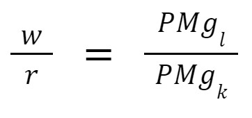
Rearranging, we find that the costs are minimal where:
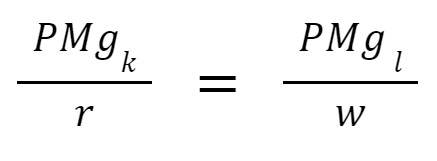
It’s easy to understand that the costs are minimal if we can distribute our budget in a way that the proportion between how much the input increases our production and its costs.
With cost minimization, the focus can be on marginal revenue. Isn’t it new that the revenue is:
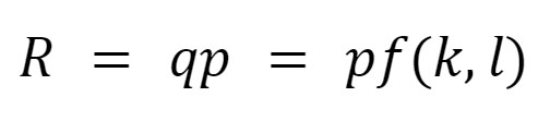
The marginal revenue is constant. It is intuitive that for each unit sold, the revenue increases the price of one unit.
An important observation is that this is true if, and only if, the firm is a price taker. Thus, the company cannot manipulate the market’s price, known as perfect competition.
With these ideas in mind, it is easy to understand profit maximization. It’s important to know that a mathematical maximum isn’t the most significant quantity but the most viable quantity to be produced. The profit formula is (economists use to denote it)
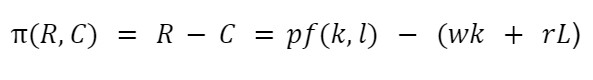
Thus, the marginal profit ('(R, C)) is:
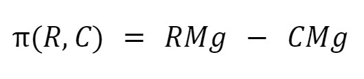
A maximum is defined as where the derivative is equal to zero, thus (R, C) where:
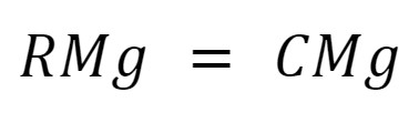
With it, the firm’s supply curve is its marginal cost.
Markets
The market is where consumers and firms interact. Each market structure has its particularities.
1. Perfect Competition: there are many consumers and producers. So, nobody can manipulate the price here, and there is no market power. There are some attributes like:
a. Homogeneous goods;
b. Symmetric information;
c. No enter or exit barriers;
d. The firms choose their supply;
e. Price takers;
f. The marginal revenue is equal to the price;
In the long run, the economic profit is zero. In the short run, some firms may be profitable, but following the assumption" 'c," the profit will attract more entrepreneurs, decreasing the prices in the long run.
2. Monopoly: only one enterprise controls the entire market, and its assumptions are:
a. Products with no substitutes;
b. The firm chooses the prices and quantities;
A monopolist firm can have economic profit in the long and short run, But as it has a price above the marginal cost, the firm can lower the price to turn away the profit-seekers, a strategic behavior.
3. Oligopoly: it's formed by a small number of big competitors. This market can behave as perfect competition when the firms don't cooperate or as a monopoly when they collaborate.
When will the firm cooperate? Economists use game theory to study when a company should make a decision, cooperate, or not. The most famous case of game theory and strategy is the prisoner dilemma.
4. Monopsony: the behavior here is almost the same as in the monopoly, but there is only one demand creator here. This demand creator can choose how much a thing will be bought and the price, but not independently.
A good example is the labor market and minimum wage policies to reduce the market power of the demand creator.
5. Oligopsony: again, the exact behavior of oligopoly, but for demanders. The demanders may choose to cooperate or not. This is what defines if the demand in this market will behave almost as in perfect competition or a monopsony.
Still using the labor market as an example, imagine a group of companies contracting their employees. They can 1) combine the wages or 2) pay as much as possible to capture all the supplies.

Researched & Authored by Luiz Eduardo
Free Resources
To continue learning and advancing your career, check out these additional helpful WSO resources:


or Want to Sign up with your social account?